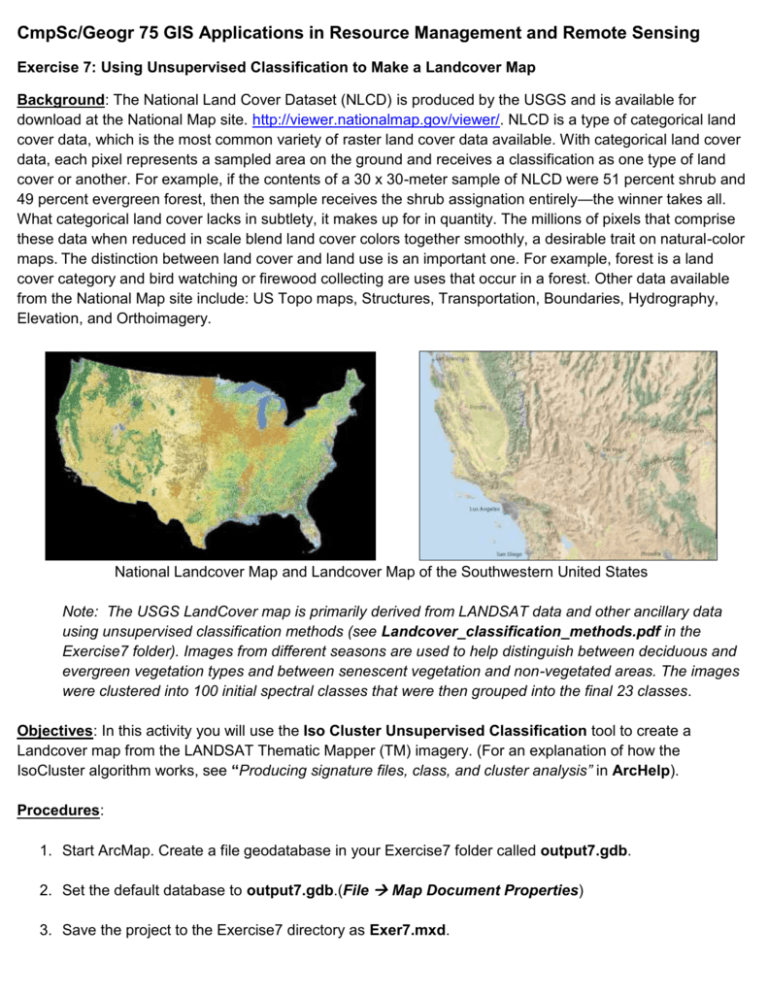
CmpSc/Geogr 75 GIS Applications in Resource Management and Remote Sensing
Exercise 7: Using Unsupervised Classification to Make a Landcover Map
Background: The National Land Cover Dataset (NLCD) is produced by the USGS and is available for
download at the National Map site. http://viewer.nationalmap.gov/viewer/. NLCD is a type of categorical land
cover data, which is the most common variety of raster land cover data available. With categorical land cover
data, each pixel represents a sampled area on the ground and receives a classification as one type of land
cover or another. For example, if the contents of a 30 x 30-meter sample of NLCD were 51 percent shrub and
49 percent evergreen forest, then the sample receives the shrub assignation entirely—the winner takes all.
What categorical land cover lacks in subtlety, it makes up for in quantity. The millions of pixels that comprise
these data when reduced in scale blend land cover colors together smoothly, a desirable trait on natural-color
maps. The distinction between land cover and land use is an important one. For example, forest is a land
cover category and bird watching or firewood collecting are uses that occur in a forest. Other data available
from the National Map site include: US Topo maps, Structures, Transportation, Boundaries, Hydrography,
Elevation, and Orthoimagery.
National Landcover Map and Landcover Map of the Southwestern United States
Note: The USGS LandCover map is primarily derived from LANDSAT data and other ancillary data
using unsupervised classification methods (see Landcover_classification_methods.pdf in the
Exercise7 folder). Images from different seasons are used to help distinguish between deciduous and
evergreen vegetation types and between senescent vegetation and non-vegetated areas. The images
were clustered into 100 initial spectral classes that were then grouped into the final 23 classes.
Objectives: In this activity you will use the Iso Cluster Unsupervised Classification tool to create a
Landcover map from the LANDSAT Thematic Mapper (TM) imagery. (For an explanation of how the
IsoCluster algorithm works, see “Producing signature files, class, and cluster analysis” in ArcHelp).
Procedures:
1. Start ArcMap. Create a file geodatabase in your Exercise7 folder called output7.gdb.
2. Set the default database to output7.gdb.(File  Map Document Properties)
3. Save the project to the Exercise7 directory as Exer7.mxd.
4. Load the six non-thermal bands from the Landsat scene from Exercise1 (Bands 1-5 and 7).
5. Load the Calaveras County NAIP image from 2010 from the Exercise7 folder. (Note: NAIP stands for
National Aerial Imagery Program, run by the USDA (United States Department of Agriculture) Farm
Service Agency. NAIP imagery is available for downloading over the Internet).
6. Load the Landcover2006 file from the Exercise 7 directory (cover2006.img).
7. Zoom to the cover2006.img layer.
8. Clip out each of the image bands loaded in Step 4 to the extent of the Data Frame by selecting them
all in the Image Analysis window, then using the clip tool (Image Analysis Window  Clip).
9. Rearrange the clipped bands so that they are in order with Band 1 at the top of the list.
10. Create a composite image from the six clipped bands. (Image Analysis  Composite).
11. Export the composite image to the output7.gdb. (Image Analysis  Export)
12. Load the Iso Cluster Unsupervised Classification script (Spatial Analyst Tools  Multivariate  Iso
Cluster Unsupervised Classification).
13. Specify the Composite layer from Step 10 as the Input raster and specify 10 output classes, then store
the classified raster in the output7.gdb. Accept the default name (“isocluster”) and take the defaults for
the remaining options (see above). Your new layer should look similar to the one below.
14. You will now create a remap table using the Reclassify Tool that defines how the values will be
reclassified (ArcToolbox  Spatial Analyst Tools Reclass  Reclassify). Before you select the
options shown below, understand that you will now reclassify the image you just reclassified and
make it simpler, modeling the National Landcover Map mentioned in the background above. Click on
and select the classified image created in Step 13 as the Swipe layer (Image Analysis—Swipe).
Use the Swipe tool along with the cover2006.img file and the Calaveras Orthophoto as reference
images to re-reclassify the 10 classes from Step 13 into these 5 groups:
1. Forest
2. Water
3. Shrub
4. Rock/Grassland/Urban
5. Other
Also use the zoom tool to zoom in and out of different areas on the map to check the accuracy of your
classifications. You will have to make some assumptions in your reasoning. Be able to support the
claims you make with evidence when reassigning each of the categories. You might wish to write
down the 5 classes above as well as the 10 classes to record which of the 10 are assigned to the 5
above. When you have decided on a solution you are comfortable with, save the output raster to the
output7.gdb. Examine the output raster for accuracy, precision, clarity, and assess/evaluate the model
of land cover you just created.
Deliverables:
1. Create a layout showing the classified image along with a legend. Export the layout to a PDF format
and print it at 8.5x11 size.
2. Submit an Abstract (~150 words) summarizing: a) the purpose of the project (1 sentence); b) the
significance (1 or 2 sentences); c) the generalized workflow (see diagram below); and d) what you
learned (~2 thirds of your Abstract, or ~100 words).
Additional Resources:
Image Classification Workflow