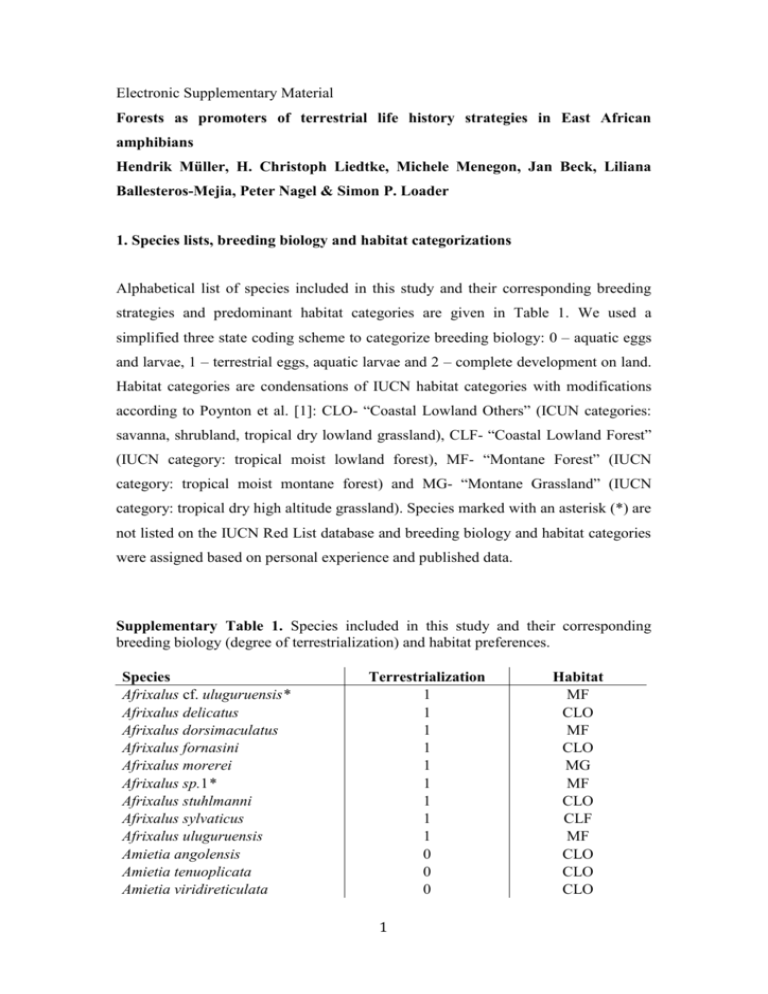
Electronic Supplementary Material
Forests as promoters of terrestrial life history strategies in East African
amphibians
Hendrik Müller, H. Christoph Liedtke, Michele Menegon, Jan Beck, Liliana
Ballesteros-Mejia, Peter Nagel & Simon P. Loader
1. Species lists, breeding biology and habitat categorizations
Alphabetical list of species included in this study and their corresponding breeding
strategies and predominant habitat categories are given in Table 1. We used a
simplified three state coding scheme to categorize breeding biology: 0 – aquatic eggs
and larvae, 1 – terrestrial eggs, aquatic larvae and 2 – complete development on land.
Habitat categories are condensations of IUCN habitat categories with modifications
according to Poynton et al. [1]: CLO- “Coastal Lowland Others” (ICUN categories:
savanna, shrubland, tropical dry lowland grassland), CLF- “Coastal Lowland Forest”
(IUCN category: tropical moist lowland forest), MF- “Montane Forest” (IUCN
category: tropical moist montane forest) and MG- “Montane Grassland” (IUCN
category: tropical dry high altitude grassland). Species marked with an asterisk (*) are
not listed on the IUCN Red List database and breeding biology and habitat categories
were assigned based on personal experience and published data.
Supplementary Table 1. Species included in this study and their corresponding
breeding biology (degree of terrestrialization) and habitat preferences.
Species
Afrixalus cf. uluguruensis*
Afrixalus delicatus
Afrixalus dorsimaculatus
Afrixalus fornasini
Afrixalus morerei
Afrixalus sp.1*
Afrixalus stuhlmanni
Afrixalus sylvaticus
Afrixalus uluguruensis
Amietia angolensis
Amietia tenuoplicata
Amietia viridireticulata
Terrestrialization
1
1
1
1
1
1
1
1
1
0
0
0
1
Habitat
MF
CLO
MF
CLO
MG
MF
CLO
CLF
MF
CLO
CLO
CLO
Amietophrynus brauni
Amietophrynus garmani
Amietophrynus gutturalis
Amietophrynus maculatus
Amietophrynus reesi
Amietophrynus xeros
Arthroleptis affinis
Arthroleptis anotis*
Arthroleptis cf. fichika*
Arthroleptis cf. xenodactyloides*
Arthroleptis fichika
Arthroleptis kidogo*
Arthroleptis lonnbergi
Arthroleptis nguruensis*
Arthroleptis nikeae
Arthroleptis reichei
Arthroleptis sp. 1*
Arthroleptis sp. 2*
Arthroleptis stenodactylus
Arthroleptis stridens
Arthroleptis tanneri
Arthroleptis xenodactyloides
Arthroleptis xenodactylus
Boulengerula boulengeri
Boulengerula cf. boulengeri*
Boulengerula cf. ulugurensis*
Boulengerula changamwensis
Boulengerula niedeni
Boulengerula taitanus
Boulengerula uluguruensis
Breviceps fichus
Breviceps mossambicus
Callulina dawida*
Callulina hanseni*
Callulina kanga*
Callulina kisiwamsitu
Callulina kreffti
Callulina laphami
Callulina shengena
Callulina meteora*
Callulina sp. 2*
Callulina sp.1*
Callulina stanleyi*
Chiromantis kelleri
Chiromantis petersii
Chiromantis xerampelina
0
0
0
0
0
0
2
2
2
2
2
2
2
2
2
2
2
2
2
2
2
2
2
2
2
2
2
2
2
2
2
2
2
2
2
2
2
2
2
2
2
2
2
1
1
1
2
MF
CLO
CLO
CLO
CLO
CLO
MF
MF
MF
MF
MF
MF
CLO
MF
MF
MF
MF
MF
CLO
CLO
MF
CLF
MF
MF
MF
MF
CLF
MF
MF
MF
MG
CLO
MF
MF
MF
MF
MF
MF
MF
MF
MF
CLF
MF
CLO
CLO
CLO
Churamiti maridadi
Hemisus marmoratus
Hildebrandtia macrotympanum
Hildebrandtia ornata
Hoplophryne cf. rogersi*
Hoplophryne cf. uluguruensis*
Hoplophryne rogersi
Hoplophryne sp. 1*
Hoplophryne uluguruensis
Hylarana galamensis
Hyperolius argus
Hyperolius cf. puncticulatus*
Hyperolius glandicolor
Hyperolius kihangensis
Hyperolius mariae
Hyperolius minutissimus
Hyperolius mitchelli
Hyperolius nasutus
Hyperolius parkeri
Hyperolius pictus
Hyperolius pseudargus
Hyperolius puncticulatus
Hyperolius pusillus
Hyperolius reesi
Hyperolius rubrovermiculatus
Hyperolius sp. 1*
Hyperolius sp. 2*
Hyperolius spinigularis
Hyperolius tanneri
Hyperolius tuberilinguis
Hyperolius viridiflavus
Kassina maculata
Kassina senegalensis
Kassina somalica
Leptopelis argenteus
Leptopelis barbouri
Leptopelis bocagii
Leptopelis cf. barbouri*
Leptopelis cf. uluguruensis*
Leptopelis concolor
Leptopelis flavomaculatus
Leptopelis parbocagii
Leptopelis parkeri
Leptopelis uluguruensis
Leptopelis vermiculatus
Mertensophryne (S.) loveridgei
NA
1
0
0
1
1
1
1
1
0
0
1
0
NA
0
0
1
0
1
1
0
1
0
0
1
NA
NA
1
NA
1
0
0
0
0
1
1
1
1
1
1
1
1
1
1
1
0
3
MF
CLO
CLO
CLO
MF
MF
MF
MF
MF
CLO
CLO
MF
CLO
MF
CLO
CLO
CLF
CLO
CLO
MG
MG
CLO
CLO
CLO
CLF
CLO
MF
MF
MF
CLO
CLO
CLO
CLO
CLO
CLO
MF
CLO
MF
MF
CLO
CLF
CLO
MF
MF
MF
CLF
Mertensophryne (S.) usambarae
Mertensophryne lindneri
Mertensophryne micranotis
Mertensophryne taitana
Mertensophryne uzunguensis
Nectophrynoides asperginis
Nectophrynoides cryptus
Nectophrynoides frontierei
Nectophrynoides laevis
Nectophrynoides laticeps
Nectophrynoides minutus
Nectophrynoides paulae
Nectophrynoides poyntoni
Nectophrynoides pseudotornieri
Nectophrynoides sp. 1*
Nectophrynoides sp. 2*
Nectophrynoides sp. 3*
Nectophrynoides sp. 4*
Nectophrynoides sp. 5*
Nectophrynoides sp. 6*
Nectophrynoides sp. 7*
Nectophrynoides tornieri
Nectophrynoides vestergaardi
Nectophrynoides viviparus
Nectophrynoides wendyae
Parhoplophryne usambarica
Petropedetes cf. yakusini*
Petropedetes martiensseni
Petropedetes yakusini
Phlyctimantis keithae
Phrynobatrachus acridoides
Phrynobatrachus breviceps
Phrynobatrachus krefftii
Phrynobatrachus mababiensis
Phrynobatrachus natalensis
Phrynobatrachus pallidus
Phrynobatrachus parvulus
Phrynobatrachus rungwensis
Phrynobatrachus scheffleri
Phrynobatrachus sp. 1*
Phrynobatrachus ukingensis
Phrynobatrachus uzungwensis
Phrynomantis bifasciatus
Probreviceps cf. durirostris*
Probreviceps durirostris
Probreviceps loveridgei
0
0
0
0
NA
2
2
2
2
2
2
2
2
2
2
2
2
2
2
2
2
2
2
2
2
NA
1
1
1
0
0
0
1
0
0
0
0
0
0
0
0
0
0
2
2
2
4
CLF
CLO
CLF
CLO
MG
MF
MF
MF
MF
MF
MF
MF
MF
MF
MF
MF
MF
MF
MF
MF
MF
MF
MF
MF
MF
MF
MF
MF
MF
MF
CLO
MG
MF
CLO
CLO
CLO
MG
MG
CLO
MG
MG
MF
CLO
MF
MF
MF
Probreviceps macrodactylus
Probreviceps rungwensis
Probreviceps uluguruensis
Ptychadena anchietae
Ptychadena grandisonae
Ptychadena mascareniensis
Ptychadena mossambica
Ptychadena oxyrhynchus
Ptychadena porosissima
Ptychadena schillukorum
Ptychadena taenioscelis
Ptychadena uzungwensis
Pyxicephalus adspersus
Pyxicephalus edulis
Schismaderma carens
Schistometopum gregorii
Scolecomorphus cf. kirkii*
Scolecomorphus cf. vittatus*
Scolecomorphus kirkii
Scolecomorphus sp.1*
Scolecomorphus uluguruensis
Scolecomorphus vittatus
Spelaeophryne methneri
Strongylopus fuelleborni
Tomopterna cryptotis
Tomopterna luganga
Xenopus borealis
Xenopus muelleri
Xenopus petersii
Xenopus victorianus
2
2
2
0
0
0
0
0
0
0
0
0
0
0
0
2
2
2
2
2
2
2
2
1
0
0
0
0
0
0
MF
MF
MF
CLO
MG
CLO
CLO
CLO
MG
CLO
CLO
MG
CLO
CLO
CLO
CLO
MF
MF
MF
MF
MF
MF
CLF
MG
CLO
CLO
MG
CLO
CLO
CLO
2. Phylogenetic Analysis
The comparative analysis outlined in this study required a species level phylogeny of
East African amphibian species. However, for the majority of species included in this
study (180 species; see Supplementary Table 1), molecular data remains unavailable.
Using existing molecular data, we explored two different strategies for producing a
comprehensive species level phylogeny of East African amphibians. Strategy 1 was to
reconstruct a genus level phylogeny of East African amphibians using a mitochondrial
and nuclear dataset. Species were added manually as a polytomy during the final tree
reconstruction step. The advantage of this approach is a complete phylogeny,
5
although with unresolved nodes and equal branch lengths among species in each
genus. While this strategy under-samples branch length differences among species, it
provides a more accurate basis for analysing species across our study area. Strategy 2
was to utilize an existing phylogeny containing species that occur across the area and
pruning out all species that do not inhabit the Eastern Arc Mountains and adjacent
lowlands. This approach provides a better estimate of species level differences, but at
the expense of completeness. Pyron and Wien [2] produced the most comprehensive
analysis of amphibian relationships and we explored the suitability of this tree, pruned
down to contain only East African taxa, to use in the comparative analyses here.
Strategy 1: Complete East African Tree
We compiled a data set for 33 amphibian ingroup species, including 30 frogs, and 3
caecilians using Genbank and previously published sequence data for the 16S rRNA
and RAG1 genes (See Supplementary Table 2). The representative samples of each
genus were not necessarily from specimens from the region. In two cases where there
was an absence of one gene fragment for a species, we produced chimeric sequences
for taxa using available sequences for presumably closely related taxa. Rag-1
sequences were not available for the following genera: Churamiti, Hildebrandtia, and
Phlyctimantis. Based on previous studies, preliminary 16S trees, or BLAST searches,
Churamiti shows closer relationships with Nectophrynoides, Hildebrandtia with
Ptychadena, and Phlyctimantis with Kassina and Rag-1 data of these genera were
used to form a chimeric sequence. In addition, analyses were conducted using
alignments with missing data, rather than using chimeric sequences (e.g. for
Churamiti, Hildebrandtia, and Phlyctimantis), to test how robust the phylogenies
including and excluding such sequences were. No significant differences were noted.
Parhoplophryne usambarica has not been collected since its original description [3]
and data on its breeding biology and phylogenetic relationships are unknown.
Therefore this taxon was excluded from all analyses.
For phylogenetic inference we sampled one lepidosaur (Lacerta lepida) as an
outgroup. The complete data set is a concatenation of one mitochondrial gene
fragment (part of the 16S rRNA gene) and one nuclear protein-coding gene fragment
(parts of Rag-1) totaling 1086 bp. Nucleotide sequences were aligned using MUSCLE
[5] with default settings in the bioinformatics tool suite Geneious Pro 5.5.4 [6].
6
Alignment ambiguities for the mitochondrial gene fragment were excluded using
GBLOCKS version 0.19b [7] with default parameter settings for block selection (less
stringent options were not selected). The resulting alignment is deposited in the Dryad
repository: http://dx.doi.org/10.5061/dryad.8f74d [4]. For each gene partition,
including codon position, the best-fit models of nucleotide substitution were identified
using the Akaike information criterion (AIC;[8]) as implemented in Modeltest version
3.7 [9]. Best-fit models were estimated for each individual partition.
The datasets were analysed using maximum likelihood (ML; [10]), and Bayesian
inference (BI; [11]). Both analyses were run using a constraint to find the optimal tree
shown in Pyron and Wiens [2], given that this represents the most comprehensive
analysis of species level relationships across all amphibians. ML analyses were
conducted with RAxML version 7.0.4 [12] using the rapid hill climbing algorithm
[13]. BI used MrBayes version 3.2.1 [14] running four simultaneous Markov chains
for 10 million generations, sampling every 1000 generations, and discarding the first
one million generations as burn-in to prevent sampling before reaching stationarity.
Two independent BI runs were performed to identify convergence. For both ML and
BI analyses, model parameters were independently optimized for each partition (‘‘unlink’’ option in effect). Support for internal branches was evaluated by nonparametric bootstrapping [10] with 1000 replicates performed with RAxML (ML),
and by posterior probabilities (BI). In order to produce a species level phylogeny for
comparative analyses, all study species were inserted in appropriate genera with interrelationships unresolved in a polytomy. This phylogeny is also deposited in the Dryad
Digital Repository as a newick file: http://dx.doi.org/10.5061/dryad.8f74d [4]. For the
BayesTraits analysis, 100 permuted trees were generated with polytomies resolved to
a branch length of 0.0001 in Mesquite v2.74 [15].
Strategy 2: Pyron and Wiens’ Tree
The phylogeny presented by Pyron and Wiens [2] is currently the most
comprehensive analysis of amphibian relationships. It includes data from 2871
species, with an average of 2563 base pairs per species. This tree was used as a basis
for conducting comparative analyses. A single Maximum likelihood tree was made
available from the authors. This tree was pruned using the R package “APE” [16],
removing all taxa not included in our analysis. The resulting tree was then used as a
7
basis for conducting the comparative analyses. Supplementary Table 3 lists species
coverage for both datasets (complete dataset and Pyron and Wiens data set).
8
Supplementary Table 2. African species used in the study with specimen-vouchers, localities, genbank accession numbers and origin.
Species
Voucher
Geographic origin
16S rRNA
RAG1
Origin
Afrixalus dorsalis
CAS 207523
Equatorial Guinea
DQ347296
DQ347236
[17]
Amietia angolensis
VUB0992
Subsaharan Africa
DQ347318
DQ347257
Genbank
Amietophrynus brauni
FMNH 251853
Tanzania
AF220886
DQ158361
[17]
Arthroleptis variabilis
CAS 207822
Equatorial Guinea
AY322263
AY364210
[17]
Boulengerula boulengeri
BMNH 2002.950
Tanzania
EF107199
EF107322
[17]
Breviceps mossambicus
VUB 1031
Subsaharan Africa
EF017947
EF018056
[17]
Callulina kreftti
TNHC 62491
Tanzania
DQ347339
DQ347281
[17]
Chiromantis rufescens
CAS “143502”
Subsaharan Africa
GQ204724
GQ204605
Genbank
Churamiti maridadi
MTSN 5584
Tanzania
FJ882769
EF107329
Genbank, RAG1 = EF107329 (N. tornieri)
Hemisus marmoratus
CAS 214843
Kenya
AY364372
AY364216
Roelants, et al 2007
Hildebrandtia ornata
“127641”
Subsaharan Africa
AF215402
DQ347245
Genbank, RAG1 = DQ347245 (Ptychadena spp)
Hoplophryne rogersi
MTSN 5158
Tanzania
EF017961
EF018050
[17]
Amnirana galamensis
VUB 0996
Subsaharan Africa
DQ347032
DQ347260
[17]
Hyperolius sp.
VUB 0924
Kenya
AF249033
AY364208
[17]
Kassina maculata
“8414”
Subsaharan Africa
AF215444
AY571651
[17]
Leptopelis kivuensis
CAS 201700
Uganda
AY322245
AY364211
[17]
Mertensophryne micranotis
BMNH 2002.343
Tanzania
EF107207
EF107330
[17]
Nectophrynoides tornieri
BMNH 2005.1375
Tanzania
EF107206
EF107329
[17]
Parhoplophryne usambarica
See MTSN 5158
Tanzania
EF017961
EF018050
[17] (assumed close H. rogersi)
Petropedetes cf. parkeri
VUB 0955
Subsaharan Africa
AY364369
AY364213
[17]
Phlyctimantis leonardi
DPL 4058 *
DQ283356 *
AY571651
Genbank, RAG1 = AY571651 (K. senegalensis)
Phrynobatrachus kreffti
VUB 1068
Tanzania
DQ347342
DQ347284
[17]
Phrynomantis bifasciatus
VUB 0541
Subsaharan Africa
AY948732
AY948918
[17]
Probreviceps macrodactylus
KMH 21399
Tanzania
AY531875
KC632525
[18]
9
Ptychadena anchietae
VUB 0958
Kenya
DQ347307
DQ347245
[17]
Pyxicephalus edulis
BMNH 2002.438
Tanzania
EF107211
EF107333
[17]
Schismaderma carens
MVZ 223386
Subsaharan Africa
DQ158424
DQ158350
Genbank
Schistometopum thomense
BMNH 2000.301
Sao Tomé
EF107204
EF107327
[17]
Scolecomorphus vittatus
CAS 168810
Tanzania
EF107171
EF107294
[17]
Spelaeophryne methneri
FMNH 255879
Tanzania
EF107167
EF107290
[17]
Strongylopus grayi
VUB 0991
Subsaharan Africa
DQ347317
DQ347256
Genbank
Tomopterna cf. natalensis
ZFMK 68815
Rep. South Africa
DQ347300
DQ347239
[17]
Xenopus cf. muelleri
VUB 0921
Kenya
AY523771
AY523743
[17]
10
3. Comparative analysis
3.1 Details on comparative trait analysis
Correlates of breeding strategy and habitat types were identified using a phylogenetic
generalized least squares approach (pGLS; [19]), using the package APE [16] in R
v.2.13.0 [20]. The regression model was constructed so as to test the effect of habitat
as a categorical, explanatory variable on the breeding biology as the response
variable, correcting for phylogenetic non-independence. Different models of
evolution were implemented as error structures in three separate regressions, allowing
traits to evolve via a Brownian Motion model, a Pagel’s λ model or an OrnsteinUhlenbeck model. AIC scores of each regression were compared and the best scoring
model was considered the most appropriate (models with ΔAIC>2 were deemed as
acceptable alternative models).
Our coding system for the breeding biology of amphibians is based on two traits:
environment of egg deposition and environment of larval development. To investigate
whether the evolution of these two traits are affected differently by the environment,
any habitat that was recovered to have a significant effect on the breeding strategy
was carried forward and correlated evolution of habitat and terrestrial ovipositioning,
and of habitat and terrestrial larval development was tested using the DISCRETE
module in BayesTraits ([21]; available at http://www.evolution.rdg.ac.uk/). This
software models the evolution of two binary traits across a given phylogeny, allowing
traits to evolve either independently or dependent of each other. Both a Likelihood
and Bayesian approach was used (see below for details). The log-likelihood scores
and harmonic means for each of the two models were then compared to test for
evidence of correlated evolution of traits.
100 trees with randomly resolved polytomies were generated in Mesquite [15] to
average the effects of varying topologies. 25 optimization attempts were used in the
likelihood analyses and significant improvements of the dependent over the
independent model (or vice versa) were measured using a log-likelihood ratio statistic
(2[(log-likelihood (dependent model) – log-likelihood (independent model))]), which
follows a χ2 distribution with 4 degrees of freedom (calculated as the difference
between the number of parameters between the two models, following Pagel [21]).
11
For the Markov chain Monte Carlo simulations, both models were run for 5 050 000
iterations, sampling every 100 chains, after a burn in period of 50 000 iterations. A
reversible-jump hyperprior with a distribution of 0 to 30 was implemented, from
which values to seed the exponential priors were drawn (rjhp exp 0 30; as
recommended by the software authors) and the ratedev was adjusted to obtain
acceptance rates between 20-40% [21]. A log-Bayes Factor (2log[harmonic mean
(dependent model)] – log[harmonic mean (independent model)]) greater than 10 was
considered as strong evidence in favour of one model over the other.
A number of different datasets were used to test the robustness of our results as
described in detail below. All datasets have been deposited in the Dryad repository:
http://dx.doi.org/10.5061/dryad.8f74d [4].
3.2 Comparison of data sets (strategies 1 and 2)
Compared to the complete dataset containing all 180 species, the phyogeny based on
Pyron and Wiens [2] contained only 73 taxa. These 73 taxa are not an accurate
representation of the four different habitat categories, with a bias in favour of Coastal
Lowland non-forest species, when compared to the 180 taxa of our dataset (see
Supplementary Table 3). For instance, whereas 50% of the species of the full dataset
are montane forest associated species, the dataset from Pyron and Wiens [2] contains
only 34.2% montane forest species. The results of the pGLS and BayesTraits analyses
using the full dataset (strategy 1) and the Pyron and Wiens data (strategy 2) were
nonetheless broadly comparable. However, only montane forest was recovered as
being significant using the Pyron and Wiens dataset, as opposed to montane and
lowland forest in our dataset.
Supplementary Table 3. Relative numbers and percentages of species included for
main habitat categories.
Pyron and Wiens [2]
No. of species
Full dataset using constrained tree
Percentage of total
number of species
No. of species
Percentage of total
number of species
CLO
42
57.5
64
35.6
CLF
3
4.1
11
6.1
12
MF
25
34.2
90
50.0
MG
3
4.1
15
8.3
Total
73
100
180
100
3.3 Results of the analyses of the full dataset (strategy 1)
Phylogenetic generalized least-squares regression implementing a Pagel’s lambda
model of evolution to test the effect of habitat on breeding biology
coefficient ± SE
t-value
p-value
1.195 ± 0.700
0.259 ± 0.080
0.159 ± 0.048
0.025 ± 0.066
1.557
3.582
4.429
0.489
p=0.121
p<0.001
p<0.001
p=0.625
Pagel’s lambda model; λ= 0.984
Intercept
Costal lowland forest
Montane forest
Montane grassland
Correlated evolution of breeding strategy and habitat in BayesTraits-DISCRETE
showing Log Likelihood scores and Harmonic Means for independent and dependent
evolution of traits
Log Likelihood
Terrestrial egg –
Montane forest
Terrestrial egg –
Coastal lowland forest
Terrestrial larva –
Montane forest
Terrestrial larva –
Coastal lowland forest
Independent
Dependent
Likelihood
Ratio
-140.556
-122.445
36.221
-92.491
-87.029
-100.574
-52.509
MCMC Harmonic mean
Independent
Dependent
Bayes
Factor
p<0.001
-145.416
-134.189
22.454
10.922
p<0.05
-104.587
-98.739
11.696
-94.318
12.512
p<0.05
-107.237
-108.125
-1.776
-52.432
0.154
p=0.997
-71.978
-69.916
4.125
p-value
3.4 Results of the analyses of the Pyron and Wiens [2] data set (strategy 2)
Phylogenetic generalized least-squares regression implementing a Pagel’s lambda
model of evolution to test the effect of habitat on breeding biology
Pagel’s lambda model; λ= 1.000
Intercept
Costal lowland forest
Montane forest
Montane grassland
coefficient ± SE
t-value
p-value
0.862 ± 0.546
0.194 ± 0.229
0.390 ± 0.116
0.020 ± 0.201
1.579
0.847
3.353
0.099
p=0.119
p=0.400
p<0.05
p=0.921
Correlated evolution of breeding strategy and habitat in BayesTraits-DISCRETE
showing Log Likelihood scores and Harmonic Means for independent and dependent
evolution of traits
Log Likelihood
Terrestrial egg –
Montane forest
Terrestrial egg –
Coastal lowland forest
Independent
Dependent
Likelihood
Ratio
-60.979
-51.705
18.549
-37.893
-37.619
0.548
13
MCMC Harmonic mean
Independent
Dependent
Bayes
Factor
p<0.001
-66.557
-60.829
11.454
p=0.969
-44.348
-44.074
0.549
p-value
Terrestrial larva –
Montane forest
Terrestrial larva –
Coastal lowland forest
-50.026
-44.101
11.850
p<0.05
-56.690
-51.221
10.938
-26.940
-25.876
2.128
p=0.712
-30.374
-31.541
-2.333
3.5 Comparison of the results of the analyses of the different datasets (strategies 1
and 2)
The overall similar results using the Pyron and Wiens tree as compared to our tree
using a resolved, genus-level phylogenetic backbone with intrageneric polytomies
shows that our phylogenetic approach is adequate for performing the comparative
analyses. The one major difference is the lack of significance for lowland forest using
the Pyron and Wiens dataset. A comparison of the datasets shows that the main
difference between the two is essentially a greatly reduced number of species
associated with lowland forests in the Pyron and Wiens dataset (3 vs. 11 in our
original dataset; see Supplementary Table 3). The lack of significance for lowland
forest for the Pyron and Wiens dataset is most likely a result of the diminished
number of lowland forest species in the dataset. In general, there are fewer lowland
forest associated species compared to the other habitat categories and this habitat is
therefore particularly sensitive to a reduction in number of species in the analysis.
Given that a comprehensive inclusion of terminals is more important for the
comparative analyses than a fully resolved tree and seeing that the results recovered
with the two datasets are comparable, we based our analyses on the full dataset
instead of using the Pyron and Wiens tree.
3.6 Correcting for undescribed species and potential taxonomic inflation
The complete data set of 180 species contains a number of not yet formally named
taxa. The overwhelming majority of these undescribed and provisionally assigned
species (all “sp.” and “cf.” taxa in Supplementary Table 1) originate from the forests
of the Eastern Arc Mountains and most are characterized by derived reproductive
modes. These species await taxonomic verification but based on current expert
opinion are putative new species (candidate species sensu [22]). Because sampling in
the region is probably biased towards montane habitats we investigated the robustness
of our analyses to the high proportion of candidate species from montane forests
compared to coastal lowlands and montane grasslands. This involved a re-analysis of
14
all data using the above approaches but with potential new species removed. This
conservative approach to species diversity estimation indicated no significant
differences in the pGLS results recovered from an analysis including all putative new
species (see results table below). In contrast to the analysis on the full dataset, the
correlation between terrestrial larval development and montane forest habitat lost
strength slightly in the BayesTraits analysis when applying a Likelihood method
(p=0.054). Similarly, the Baysian method could no longer recover a significant
improvement of the dependent over the independent model of evolution for terrestrial
egg deposition in association with Coastal Lowland Forest (BF=7.180).
After removing candidate species the pGLS results continue to show a
significant positive effect of both forest types on the occurrence of terrestrial breeding
amphibians and the conclusions drawn from the BayesTraits analysis are comparable
too: there is support for correlated evolution of terrestrial egg deposition
predominantly with montane forest but also with coastal lowland forest. Although
there is some indication of correlated evolution of terrestrial larval development and
montane forest, this association is no longer statistically supported.
Phylogenetic generalized least-squares regression implementing a Pagel’s lambda
model of evolution to test the effect of habitat on breeding biology
Pagel’s lambda model; λ= 0.981
Intercept
Costal lowland forest
Montane forest
Montane grassland
coefficient ± SE
t-value
p-value
1.204 ± 0.778
0.257 ± 0.082
0.227 ± 0.063
0.040 ± 0.069
1.547
3.133
3.611
0.575
p=0.124
p<0.05
p<0.001
p=0.566
Correlated evolution of breeding strategy and habitat in BayesTraits-DISCRETE
showing Log Likelihood scores and Harmonic Means for independent and dependent
evolution of traits
Log Likelihood
Terrestrial egg –
Montane forest
Terrestrial egg – Coastal
lowland forest
Terrestrial larva –
Montane forest
Terrestrial larva –
Coastal lowland forest
MCMC Harmonic mean
Independen
Dependent
t
Independent
Dependent
Likelihood
Ratio
-121.202
-108.468
25.469
p<0.001
-126.885
-118.146
17.478
-84.914
-80.013
9.802
p<0.05
-99.555
-95.965
7.180
-84.156
-79.515
9.281
p=0.054
-90.569
-93.368
-5.598
-47.868
-47.870
-0.005
p=1.000
-68.501
-66.581
3.840
15
p-value
Bayes
Factor
3.7 Influence of viviparous species
Both viviparity and ovoviviparity are highly derived reproductive modes that are
generally rare among amphibians [23]. Within East Africa the caecilian genera
Scolecomorphus and Schistometopum contain viviparous species [24] and the bufonid
Nectophrynoides species are ovoviviparous [23]. When looking at the taxonomic
composition of lowland forest and non-forest habitats, montane forest, and montane
grassland, it is apparent that viviparous and ovoviviparous species are predominantly
found in montane forest. Especially Nectophrynoides represents a species-rich
radiation of small bufonids nearly exclusively confined to the montane forests of the
EAM. To test the influence that viviparous and ovoviviparous species might have on
the analyses, we performed a separate pGLS and BayesTraits analysis excluding
viviparous and ovoviviparous species from the dataset. Both montane and lowland
forest habitats were again recovered as containing significantly more species with
terrestrialized breeding strategies than the other habitat categories for the pGLS
analysis. In comparison to the results when using the full dataset, the BayesTraits
analysis no longer recovers a significant association for terrestrial larval development
and montane forest (LR=6.056; p=0.195). Furthermore the MCMC method could no
longer recover a significant improvement of the dependent over the independent
model of evolution for terrestrial egg deposition in association with coastal lowland
forest although the log Bayes Factor is only marginally below the significance
threshold (BF=9.218).
As is the case for the analyses using the conservative dataset (above), the
pGLS and BayesTraits analysis suggest that even when removing the viviparous
lineages, the general association of terrestrial breeding with forest habitat (especially
montane forest) remains significant. However, no statistically significant support
could be found for correlated evolution of terrestrial larval development and either
forest habitat types. Given the relatively high number of viviparous and
ovoviviparous species in the original dataset, the latter result is not surprising.
Phylogenetic generalized least-squares regression implementing a Pagel’s lambda
model of evolution to test the effect of habitat on breeding biology
Pagel’s lambda model; λ= 0.969
Intercept
Costal lowland forest
Montane forest
16
coefficient ± SE
t-value
p-value
0.994 ± 0.676
0.256 ± 0.078
0.224 ± 0.057
1.470
3.259
3.957
p=0.144
p<0.05
p<0.001
Montane grassland
0.040 ± 0.067
0.601
p=0.549
Correlated evolution of breeding strategy and habitat in BayesTraits-DISCRETE
showing Log Likelihood scores and Harmonic Means for independent and dependent
evolution of traits
Log Likelihood
Terrestrial egg –
Montane forest
Terrestrial egg –
Coastal lowland forest
Terrestrial larva –
Montane forest
Terrestrial larva –
Coastal lowland forest
Independent
Dependent
Likelihood
Ratio
-130.676
-113.450
34.452
-88.566
-83.007
-89.472
-47.361
MCMC Harmonic mean
Independent
Dependent
Bayes
Factor
p<0.001
-139.213
-126.319
25.788
11.117
p<0.05
-102.530
-97.921
9.218
-86.444
6.056
p=0.1950
-97.720
-98.569
-1.699
-46.838
1.046
p=0.9027
-66.991
-63.776
6.429
p-value
References
1.
Poynton J.C., Loader S.P., Sherratt E., Clarke B.T. 2007 Amphibian diversity
in east african biodiversity hotspots: Altitudinal and latitudinal patterns. Biodivers
Conserv 16(4), 1103-1118. (doi:10.1007/s10531-006-9074-1).
2.
Pyron R.A., Wiens J.J. 2011 A large-scale phylogeny of Amphibia including
over 2800 species, and a revised classification of extant frogs, salamanders, and
caecilians. Mol Phylogenet Evol 61(2), 543-583. (doi:10.1016/j.ympev.2011.06.012).
3.
Barbour T., Loveridge A. 1928 A comparative study of the herpetological
faunae of the Uluguru and Usambara Mountains, Tanganyika Territory, with
descriptions of new species. Memoirs of the Museum of Comparative Zoology 50, 85265.
4.
Müller H., Liedtke H.C., Menegon M., Beck J., Ballesteros-Mejia L., Nagel
P., Loader S.P. 2013 Data from: Forests as promoters of terrestrial life history
strategies
in
East
African
amphibians.
Dryad
Digital
Repository
http://dx.doi.org/10.5061/dryad.8f74d.
5.
Edgar R.C. 2004 MUSCLE: multiple sequence alignment with high accuracy
and high throughput. Nucleic Acids Res 32(5), 1792-1797. (doi:10.1093/nar/gkh340).
6.
Drummond A.J., Ashton B., Buxton S., Cheung M., Cooper A., Duran C.,
Field M., Heled J., Kearse M., Markowitz S., et al. 2012 Geneious v5.6. (Available
from http://www.geneious.com.
7.
Castresana J. 2000 Selection of Conserved Blocks from Multiple Alignments
for Their Use in Phylogenetic Analysis. Molecular Biology and Evolution 17(4), 540552.
8.
Akaike H. 1974 A new look at the statistical model identification. IEEE
Transactions on Automatic Control 19, 716-723.
9.
Posada D., Crandall K.A. 1998 Modeltest: Testing the model of DNA
substitution. Bioinformatics 14, 817-818.
10.
Felsenstein J. 1985 Confidence-limits on phylogenies - an approach using the
bootstrap. Evolution 39, 783-791.
11.
Huelsenbeck J.P., Ronquist F., Nielsen R., Bollback J.P. 2001 Bayesian
Inference of Phylogeny and Its Impact on Evolutionary Biology. Science 294(5550),
2310-2314. (doi:10.1126/science.1065889).
17
12.
Stamatakis A. 2006 RAxML-VI-HPC: maximum likelihood-based
phylogenetic analyses with thousands of taxa and mixed models. Bioinformatics
22(21), 2688-2690. (doi:10.1093/bioinformatics/btl446).
13.
Stamatakis A., Hoover P., Rougemont J. 2008 A Rapid Bootstrap Algorithm
for the RAxML Web Servers. Systematic Biology 57(5), 758-771.
(doi:10.1080/10635150802429642).
14.
Ronquist F., Teslenko M., van der Mark P., Ayres D.L., Darling A., Höhna S.,
Larget B., Liu L., Suchard M.A., Huelsenbeck J.P. 2012 MrBayes 3.2: Efficient
Bayesian Phylogenetic Inference and Model Choice across a Large Model Space.
Systematic Biology. (doi:10.1093/sysbio/sys029).
15.
Maddison W.P., Maddison D.R. 2010 Mesquite: A modular system for
evolutionary analysis. Version 2.74. http://mesquiteproject.org.
16.
Paradis E., Claude J., Strimmer K. 2004 APE: analyses of phylogenetics and
evolution in R language. Bioinformatics 20, 289-290.
17.
Roelants K., Gower D.J., Wilkinson M., Loader S.P., Biju S.D., Guillaume K.,
Moriau L., Bossuyt F. 2007 Global patterns of diversification in the history of modern
amphibians. Proceedings of the National Academy of Sciences 104(3), 887-892.
(doi:10.1073/pnas.0608378104).
18.
Loader S.P., Poynton J.C., Mariaux J. 2004 Herpetofauna of Mahenge
Mountain, Tanzania: a window on African biogeography. Afr Zool 39(1), 71-76.
19.
Martins E.P., Hansen T.F. 1997 Phylogenies and the comparative method: a
general approach to incorporating phylogenetic information into the analysis of
interspecific data. Am Nat (149), 646-667.
20.
R Core Team. 2012 R: a language and enviroment for statistical computing. R
foundation for statistical computing. (http://www.R-project.org/).
21.
Pagel M. 1994 Detecting correlated evolution on phylogenies: a general
method for the comparative analysis of discrete characters. Proceedings of the Royal
Society B - Biological Sciences 255, 37-45.
22.
Vences M., Wake D. 2007 Speciation, species boundaries and phylogeography
of amphibians. In Amphibian biology volume 7: Systematics (eds. Heatwole H., Tyler
M.), p. 570, Surrey Beatty & Sons.
23.
Wake M.H. 1978 The Reproductive Biology of Eleutherodactylus jasperi
(Amphibia, Anura, Leptodactylidae), with Comments on the Evolution of LiveBearing Systems. Journal of Herpetology 12(2), 121-133. (doi:10.2307/1563398).
24.
Wilkinson M., Nussbaum R.A. 2006 Phylogeny and classification of
caecilians. In Reproductive biology and phylogeny of Gymnophiona (ed. Exbrayat J.M.), pp. 527-612. Enfield, Science Publishers.
18