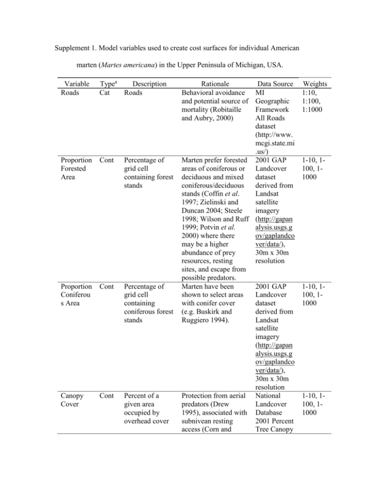
Supplement 1. Model variables used to create cost surfaces for individual American
marten (Martes americana) in the Upper Peninsula of Michigan, USA.
Variable
Roads
Typea
Description
Cat
Roads
Proportion
Forested
Area
Cont
Percentage of
grid cell
containing forest
stands
Proportion
Coniferou
s Area
Cont
Percentage of
grid cell
containing
coniferous forest
stands
Canopy
Cover
Cont
Percent of a
given area
occupied by
overhead cover
Rationale
Behavioral avoidance
and potential source of
mortality (Robitaille
and Aubry, 2000)
Data Source
MI
Geographic
Framework
All Roads
dataset
(http://www.
mcgi.state.mi
.us/)
Marten prefer forested 2001 GAP
areas of coniferous or Landcover
deciduous and mixed
dataset
coniferous/deciduous
derived from
stands (Coffin et al.
Landsat
1997; Zielinski and
satellite
Duncan 2004; Steele
imagery
1998; Wilson and Ruff (http://gapan
1999; Potvin et al.
alysis.usgs.g
2000) where there
ov/gaplandco
may be a higher
ver/data/),
abundance of prey
30m x 30m
resources, resting
resolution
sites, and escape from
possible predators.
Marten have been
2001 GAP
shown to select areas
Landcover
with conifer cover
dataset
(e.g. Buskirk and
derived from
Ruggiero 1994).
Landsat
satellite
imagery
(http://gapan
alysis.usgs.g
ov/gaplandco
ver/data/),
30m x 30m
resolution
Protection from aerial National
predators (Drew
Landcover
1995), associated with Database
subnivean resting
2001 Percent
access (Corn and
Tree Canopy
Weights
1:10,
1:100,
1:1000
1-10, 1100, 11000
1-10, 1100, 11000
1-10, 1100, 11000
Raphael 1992), and
prey (Thompson and
Colgan 1994)
Fisher
Harvest
Density
a
Cont
Density of
harvested fishers
dataset
(http://www.
mrlc.gov/nlc
d2001.php),
30m x 30m
resolution
Fisher may predate on Derived from 1-10, 1marten (Raine 1987)
Michigan
100, 1and represent a source Department
1000
of indirect competition of Natural
for food resources,
Resources
particularly small
fisher harvest
mammal prey (Krohn locations
et al. 1997) and
during 2000denning sites (Clem
2004 and
1977).
ESRI
ArcGIS 9.3
Kernel
Density Tool
Cont = Continuous, Cat = Categorical.
5
Buskirk SW, Ruggiero LF (1994) American marten. In: Ruggiero LF, Aubry KB,
Buskirk SW, Lyon LJ, Zielinski WJ, (ed) The scientific basis for conserving
forest carnivores: American marten, fisher, lynx, and wolverine in the western
United States. Gen. Tech. Rep. RM-254. Fort Collins, CO: US. Department of
10
Agriculture, Forest Service, Rocky Mountain Forest and Range Experiment
Station. pp7-37
Clem MK (1977) Interspecific relationship of fisher and marten in Ontario during winter.
In: Philips RL, Jonkel C (ed) Proceedings of the 1975 predator symposium,
Missoula, MT, 16-19 June 1975. Montana Forest Conservation Experiment
15
Station, University of Montana, Missoula. pp165-182
Coffin KW, Kujala QJ, Douglass RJ, Irby LR (1997) Interactions among marten prey
availability, vulnerability, and habitat structure. Martes: taxonomy, ecology,
techniques, and management. The Provincial Museum of Alberta, Edmonton,
Alberta, Canada, pp199–210
20
Corn JG, Raphael MG (1992) Habitat characteristics at marten subnivean access sites. J
Wildlife Manage 56:442–448
Drew GS (1995) Winter habitat selection by American marten (Martes americana) in
Newfoundland: why old growth? PhD thesis, Utah State University
Krohn WB, Zielinski WJ, Boone RB (1997) Relations among fishers, snow, and martens
25
in California: results from small-scale spatial comparisons. Martes: taxonomy,
ecology, techniques, and management. Provincial Museum of Alberta, Edmonton,
Alberta, pp211–232
Potvin F, Belanger L, Lowell K (2000) Marten habitat selection in a clearcut boreal
landscape. Conserv Biol 14:844-857
30
Raine RM (1987) Winter food habits and foraging behaviour of fishers (Martes pennanti)
and martens (Martes americana) in southeastern Manitoba. Can J Zool 65:745–747
Robitaille JF, Aubry K (2000) Occurrence and activity of American martens Martes
americana in relation to roads and other routes. Acta Theriol 45:137–143
Steele MA (1998) Tamiasciurus hudsonicus. Mammalian Species, American Society of
35
Mammalogists, pp1-9
Thompson ID, Colgan PW (1994) Marten activity in uncut and logged boreal forests in
Ontario. J Wildl Manage 58:280–288
Wilson EBDE, Ruff S (1999) North American I Mammals. Smithsonian Institute,
Washington, DC, USA
40
Zielinski WJ, Duncan NP. (2004) Diets of sympatric populations of American martens
(Martes americana) and fishers (Martes pennanti) in California. J Mamm 85:470–
477
45
Supplement 2. Hypothesized cost of American marten (Martes americana) movement in
50
the upper peninsula of Michigan, USA in relation to marten harvest location and
affiliation to one of three genetic clusters (indicated with different symbols). Cost
surfaces represent a) presence of roads, b) canopy cover, c) percent forested area, d)
percent coniferous forest, and e) fisher (Pekania pennanti) harvest density. Variables are
described in Supplement 1.
55
Supplement 3. Results from sensitivity analysis to determine the influence of weighting
scheme on the resulting cost distance from least cost path (LCP) analysis for each
landscape feature.
Model
Geographic Distance (Euc)
Roads (2 levels) (Rd)
Canopy Cover (Can)
Proportion Forested Area (For)
Fisher Density (PP)
Proportion Coniferous Area
(Con)
60
Weights
1
1, 10
1,100
1, 1000
1 to 10
1 to 100
1 to 1000
1 to 10
1 to 100
1 to 1000
1 to 10
1 to 100
1 to 1000
1 to 10
1 to 100
1 to 1000
Mantel
r
0.209
0.224
0.216
0.223
0.190
0.211
0.185
0.184
0.208
0.052
0.198
0.192
0.162
P
value
<0.002
<0.002
<0.002
<0.002
<0.002
<0.002
<0.002
<0.002
<0.002
0.035
<0.002
<0.002
<0.002
0.243 <0.002
0.221 <0.002
0.245 <0.002
Supplement 4: Description of Causal Modeling methods. We used causal modeling
(Cushman et al. 2006; Cushman and Landguth 2010b) based on partial Mantel tests to
quantify support (Mantel r) for each of our models and to inform our boundary analysis
(described in Supplement 5) by identifying the landscape variables (given the set of
65
variables we quantified) that most highly correlated with genetic relatedness (Smouse et
al. 1986; Cushman et al. 2006. We assessed statistical significance of each partial Mantel
test at α = 0.0021 (Bonferonni correction of α = 0.05 based on multiple model
comparisons). We conducted a series of partial Mantel tests between genetic distance and
least cost distance corresponding to each of our landscape hypotheses, after partialing out
70
Euclidean distance (e.g., Genetic Distance ~ Cost Distance from Model 1 | Euclidean
Distance; Cushman et al. 2006). We also conducted a series of partial Mantel tests
between genetic distance and Euclidean distance, partialing out the least cost distance
corresponding to each of our landscape hypotheses (e.g., Genetic Distance ~ Euclidean
Distance | Cost Distance from Model 1). If cost distance estimated based on one or more
75
landscape features was significantly associated with genetic distance independent of
Euclidean distance, we expected the former test to be statistically significant and the
latter to be not significant (Cushman et al. 2006).
Cushman SA, McKelvey KS, Hayden J, Schwartz MK (2006) Gene flow in complex
landscapes: testing multiple hypotheses with causal modeling. Am Nat 168:486–
80
499
Cushman SA, Landguth EL (2010b) Spurious correlations and inference in landscape
genetics. Mol Ecol 19:3592-3602
Smouse PE, Long JC, Sokal RR (1986) Regression and Correlation Extensions of the
Mantel Test of Matrix Correspondence. Syst Zool 35:627-632
85
Supplement 5: Defining genetic clusters (additional details)
The clustering algorithm implemented in program Geneland incorporates the
spatial coordinates of the multilocus genotype for each individual to determine posterior
probabilities of membership to a genetic cluster. We defined the boundaries of genetic
90
clusters as sharp gradients in posterior probabilities among different clusters. We
assumed that the locational error associated with marten harvest location reporting was
randomly distributed around the centroid of each township section (1 section = 2.6 km2),
and included coordinate uncertainty of 1 km associated with marten harvest locations.
We estimated the number of genetic clusters (K) using a Markov Chain Monte
95
Carlo (MCMC) algorithm. We first allowed K to vary and subsequently ran the algorithm
with K fixed at the value most supported by the data (i.e., K from the initial run with the
highest average posterior probability; Guillot et al. 2005b). We iterated this process four
times with the following parameters: 250,000 MCMC iterations, maximum rate of
Poisson process at 495 (i.e., equal to the number of individuals as suggested by Guillot et
100
al. 2005a), minimum K = 1, maximum K = 5, and maximum number of nuclei of the
Poisson-Voronoi tessellation at approximately 3 times the maximum rate of the Poisson
process (Guillot et al. 2005b). We used an uncorrelated allele frequency model (Guillot et
al. 2005a). We calculated the mean logarithm of the posterior probability by re-running
the MCMC algorithm 10 times (thinning = 10) with K fixed at 3 (previously inferred
105
number of genetic clusters when allowing K to vary).
Guillot G, Estoup A, Mortier F, Cosson JF (2005b) A spatial statistical model for
landscape genetics. Genetics 170:1261–1280
Supplement 6: Mantel and partial Mantel tests, comparing the relative influence of
landcover variables in predicting American marten (Martes americana) gene flow.
110
Significant partial Mantel results are in bold.
Mantel
partial Mantel2
Model1
r
P
r
P3
Con + Rd
0.226 <0.002
0.076 <0.002
Con
0.221 <0.002
0.056 <0.002
Can + Con
0.220 <0.002
0.055 <0.002
Rd
0.216 <0.002
0.037 <0.002
Can + Con + Rd
0.220 <0.002
0.056 0.004
Con + PP
0.219 <0.002
0.053 0.004
PP + Rd + Con
0.220 <0.002
0.052 0.004
Can + Con + PP +
0.218 <0.002
0.046 0.004
Rd
Can + Con + PP
0.218 <0.002
0.045 0.006
PP
0.192 <0.002
0.028 0.076
Can
0.211 <0.002
-0.021 0.093
Can + PP
0.208 <0.002
-0.017 0.127
PP + Rd
0.201 <0.002
0.019 0.135
Can + Rd
0.210 <0.002
-0.017 0.158
PP + Rd + For
0.209 <0.002
-0.017 0.166
Can + For + Rd
0.209 <0.002
-0.017 0.171
PP + Rd + Can
0.209 <0.002
-0.015 0.176
Can + For
0.208 <0.002
-0.017 0.181
For + PP
0.197 <0.002
-0.017 0.211
Can + For + PP
0.209 <0.002
-0.010 0.292
Can + For + PP +
0.210 <0.002
-0.008 0.298
Rd
For
0.208 <0.002
0.010 0.314
For + Rd
0.212 <0.002
0.007 0.323
Euc
0.209 <0.002
NA
NA
1
Euc = Euclidean distance, Rd = Roads, Con = Proportion of coniferous forest, For=
Proportion of area that is forested, PP = Fisher (Pekania pennanti) density, Can = Canopy
cover.
2
115
Partial Mantel tests quantify the residual variation between each model and genetic
distance, after accounting for variation associated with Euclidean distance (e.g., Can +
Con | Euc).
3
Bonferroni correction of α = 0.05/24 = 0.0021).
All univariate Mantel models correlating genetic relatedness to least cost paths were
significant, with the highest Mantel r value corresponding to the model that included Con
120
+ Rd (r = 0.226, P < 0.002; Supplement 6). After accounting for the variation associated
with Euclidean distance (Euc) using partial Mantel tests, we found 4 significant models
that described the boundaries of genetic relatedness (α < 0.0021): 1) Coniferous, 2) Roads
3) Canopy + Coniferous, and 4) Coniferous + Roads (Supplement 6). Additionally, the
relationship between genetic relatedness and Euclidean distance was not significant after
125
partialing out the variation associated with each of the above 4 models (Supplement 7).
The Coniferous + Roads model had the most support compared to all alternative models
based on the magnitude of the partial Mantel r values (Supplement 6).
Supplement 7. Partial Mantel tests comparing the relative influence of several landcover
130
variables in predicting American marten (Martes americana) gene flow. Significant
partial Mantel results are in bold.
partial Mantel
P
Euc | PP
0.10
<0.002
Euc | For + PP
0.09
<0.002
Euc | PP + Rd
0.08
<0.002
Euc | For
0.05
<0.002
Euc | Can + For
0.05
<0.002
Euc | PP + Rd + Can
0.05
<0.002
Euc | Can + For + PP
0.05
<0.002
Euc | Can + For + Rd
0.05
<0.002
Euc | Can + PP
0.05
0.003
Euc | Can + Rd
0.05
0.005
Euc | Can + For + PP + Rd
0.04
0.005
Euc | PP + Rd + For
0.05
0.006
Euc | Can
0.04
0.007
Euc | Rd
-0.02
0.017
Euc | For + Rd
0.03
0.041
Euc | Con + PP
0.02
0.086
Euc | Can + Con + Rd
-0.02
0.098
Euc | Can + Con
-0.02
0.124
Euc | PP + Rd + Con
0.02
0.172
Euc | Can + Con + PP + Rd
-0.02
0.197
Euc | Con + Rd
-0.01
0.222
Euc | Can + Con + PP
-0.01
0.237
Euc | Con
-0.01
0.351
1
Partial Mantel tests quantify the residual variation between Euclidean distance and
Model1
r
genetic distance, after accounting for variation associated with each alternative landscape
model.
135
2
Bonferroni correction of α = 0.05/24 = 0.0021)