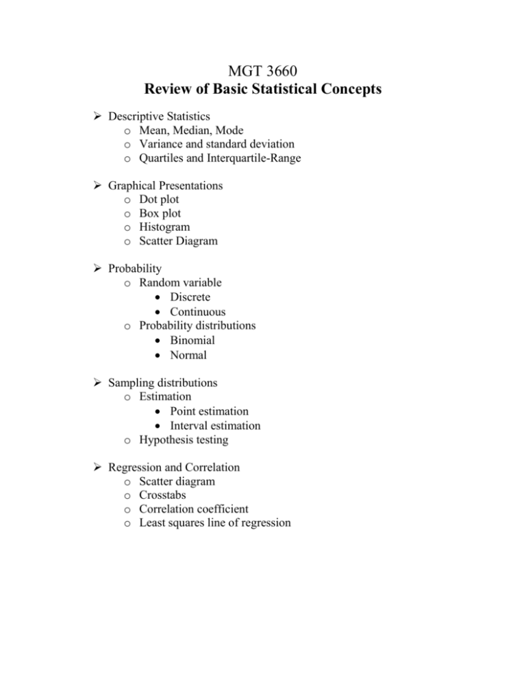
MGT 3660
Review of Basic Statistical Concepts
 Descriptive Statistics
o Mean, Median, Mode
o Variance and standard deviation
o Quartiles and Interquartile-Range
 Graphical Presentations
o Dot plot
o Box plot
o Histogram
o Scatter Diagram
 Probability
o Random variable
 Discrete
 Continuous
o Probability distributions
 Binomial
 Normal
 Sampling distributions
o Estimation
 Point estimation
 Interval estimation
o Hypothesis testing
 Regression and Correlation
o Scatter diagram
o Crosstabs
o Correlation coefficient
o Least squares line of regression
Excel Commands and Functions
Statistical Commands in Excel
Data/Pivot Table
Develop frequency distributions and histograms
Tools/Data Analysis
 Descriptive Statistics
 Correlation
 Regression
Statistical Functions in Excel
Descriptive
Statistics
AVERAGE
TRIMMEAN
MEDIAN
PERCENTILE
QUARTILE
VAR.S
STDEV.S
Probability
Distributions
BINOMDIST
NORM.DIST
NORM.INV
NORM.S.DIST
NORM.S.INV
Hypothesis testing
T.DIST
T.DIST.2T
T.DIST.RT
T.INV
T.INV.2T
T.TEST
CONFIDENCE.T
Regression and
correlation
CORREL
SLOPE
INTERCEPT
FORECAST
TREND
Example: TRIMMEAN(Array, percent)
TRIMMEAN: This function calculates the trimmed mean for a list of numbers.
Parameters:
Array: Range of numerical values to trim and average
Percent: A value between 0 and 1; represents the fractional number of values to
exclude from the range of data. For example, if percent = 0.2, and the
Array contains 20 cell values, 20 x .2 = 4 data values will be trimmed, two
smallest values and two largest values.
Creating a Box Plot
1.
Set up the following data for the plot
 Maximum - Q3
 Q3 – Median
 Median - Q1
 Q1
 Q1-Minimum
(Note: Q1 = First quartile, Q3 = Third quartile)
2.
3.
4.
5.
6.
7.
8.
9.
10.
11.
12.
13.
14.
15.
Highlight the middle three values from above (do not highlight all 5 values).
Click Insert, and from the “Charts” section, select Column/2D stacked
Column bar graph.
Click “Switch Row/Column”
Delete (i) the legend label and (ii) X-axis label
Select the Graph, click Select Data and rearrange series 1, series 2 and series 3
in the proper order
Select the bottom stack. Click “Layout”, “Error bars”, “More Error Bar
options”
Select “Minus”, “Custom”, and then click “Specify Value”
Select “Negative Error Value” and enter the cell address of Q1-Minimum
value. Then click OK and “Close”.
Select the bottom bar. Then right click and select “Format Data Series”
Select “Fill” and check “No Fill”. Then click “Close”
Select the top stack. Click “Layout”, “Error bars”, “More Error Bar options”
Select “Plus”, “Custom”, and then click “Specify Value”
Select “Positive Error Value” and enter the cell address of Maximum-Q3
value. Then click OK and “Close”.
Add a chart title and resize it.
Probability Distributions
Random Variable (RV): A numerical description of the outcome of an experiment.
Discrete RV: A random variable that can take a countable set of values. For
instance, if an experiment consists of inspecting 10 laptops produced by a
manufacturer, then a random variable X can be defined as the number of defective
laptops in the lot. The possible values for X are any number from zero to 10.
Continuous RV: A random variable that can take an uncountable range of values.
For instance, if an experiment consists of measuring the amount of toothpaste in a
6 oz. tube, then a random variable X can be defined as the amount of toothpaste in
a tube. The possible values for X could be any value between 5.8 oz. To 6.2 oz.
The values within the range is not countable.
Probability Distribution: A description of how the probabilities are distributed over the
values the random variable can assume.
Expected Value: The expected value of a RV is the average value of the RV if the
experiment is repeated over a long run.
Expected Value of a Discrete Random Variable: E(x) = µ =  (x f(x))
Normal Probability Distribution: A continuous probability distribution. The normal
distribution is a symmetrical distribution with a mean, , and a standard deviation, .

Example
The ticket sales for events held at the new civic center are believed to be normally
distributed with a mean of 12,000 and a standard deviation of 1,000.
a.
What is the probability of selling no more than 8,000 tickets?
b. What is the probability of selling more than 10,000 tickets?
c.
What is the probability of selling between 9,500 and 11,000 tickets?
d. How many tickets will have a probability of selling of 98% ?
Confidence Interval and Hypothesis Testing


Simple Random Sample
Point Estimation:
Size
Mean
Standard deviation

(Point Estimator)
Sample Statistic
Population Parameter
n
N
S


Sampling Error = | –  |
Confidence Interval
  x  t 2 .
S
n
(Use Z instead of t only if  is known)
Hypothesis Testing
1.
2.
3.
4.
Set up the null and the alternative hypotheses.
Compute p-value for rejecting the null-hypothesis using t-distribution (Use Z
instead of t only if  is known)
X  0
Use t 
to determine the p-value.
S n
If p-value <= , then reject the null-hypothesis; otherwise do not reject.
Interpret and report the results
Correlation and Simple Regression
Coefficient of Correlation r:
Correlation coefficient between two sets of data (X and Y) is a number between -1 and 1.
It measures the strength and direction of linear association between the two sets of data of
equal size.
The sign indicates the direction of the association. Positive numbers indicate direct
association and negative numbers indicate inverse relationship.
The value indicates the strength of the association between the two data sets. A number
close to 1 or -1 indicates strong relationship. A number to close to zero indicates weak or
non-existent relationship.
Formula for determining correlation coefficient:
r=
(x i  x )(y i  y )
2
2
 (x i  x )  (y i  Y )
Simple Linear Regression
Simple linear regression equation is a linear function between two data sets of equal size,
of the form Y = b0 + b1X, where, y = dependent variable and x = independent variable.
The model: Y = b0 + b1X + e,
where, b0 = the y-intercept, b1 = the slope of the line, and e = error
The model may be written as Y = Ŷ + e, where Ŷ = estimated value of Y
Then estimation error = e = Y – Ŷ, and squared error = (Y – Ŷ)2
The following formulas give estimates for b0 and b1 that minimizes the squared sum of
estimation error, called least squared estimates.
( x i  x )( y i  y)
b o  y  b1 x
b1 
2
 (x i  x)
Excel functions for regression:
b1 = SLOPE(y-range,x-range)
b0 = INTERCEPT(y-range,x-range)
Ŷ = FORECAST(y-range,x-range,Given x-value)
Ŷ = TREND (Given x-value,y-range,x-range)