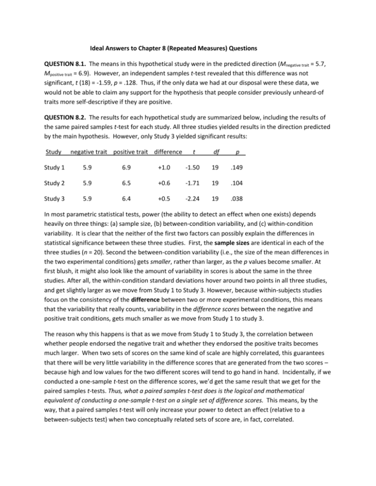
Ideal Answers to Chapter 8 (Repeated Measures) Questions
QUESTION 8.1. The means in this hypothetical study were in the predicted direction (Mnegative trait = 5.7,
Mpositive trait = 6.9). However, an independent samples t-test revealed that this difference was not
significant, t (18) = -1.59, p = .128. Thus, if the only data we had at our disposal were these data, we
would not be able to claim any support for the hypothesis that people consider previously unheard-of
traits more self-descriptive if they are positive.
QUESTION 8.2. The results for each hypothetical study are summarized below, including the results of
the same paired samples t-test for each study. All three studies yielded results in the direction predicted
by the main hypothesis. However, only Study 3 yielded significant results:
Study
negative trait positive trait difference
t
df
p .
Study 1
5.9
6.9
+1.0
-1.50
19
.149
Study 2
5.9
6.5
+0.6
-1.71
19
.104
Study 3
5.9
6.4
+0.5
-2.24
19
.038
In most parametric statistical tests, power (the ability to detect an effect when one exists) depends
heavily on three things: (a) sample size, (b) between-condition variability, and (c) within-condition
variability. It is clear that the neither of the first two factors can possibly explain the differences in
statistical significance between these three studies. First, the sample sizes are identical in each of the
three studies (n = 20). Second the between-condition variability (i.e., the size of the mean differences in
the two experimental conditions) gets smaller, rather than larger, as the p values become smaller. At
first blush, it might also look like the amount of variability in scores is about the same in the three
studies. After all, the within-condition standard deviations hover around two points in all three studies,
and get slightly larger as we move from Study 1 to Study 3. However, because within-subjects studies
focus on the consistency of the difference between two or more experimental conditions, this means
that the variability that really counts, variability in the difference scores between the negative and
positive trait conditions, gets much smaller as we move from Study 1 to study 3.
The reason why this happens is that as we move from Study 1 to Study 3, the correlation between
whether people endorsed the negative trait and whether they endorsed the positive traits becomes
much larger. When two sets of scores on the same kind of scale are highly correlated, this guarantees
that there will be very little variability in the difference scores that are generated from the two scores –
because high and low values for the two different scores will tend to go hand in hand. Incidentally, if we
conducted a one-sample t-test on the difference scores, we’d get the same result that we get for the
paired samples t-tests. Thus, what a paired samples t-test does is the logical and mathematical
equivalent of conducting a one-sample t-test on a single set of difference scores. This means, by the
way, that a paired samples t-test will only increase your power to detect an effect (relative to a
between-subjects test) when two conceptually related sets of score are, in fact, correlated.
QUESTION 8.3. The proper analysis for these data is a mixed model ANOVA in which trait favorability is
the within-subjects variable and self-esteem is the between-subjects variable. In addition to a significant
main effect of trait favorability, F (1, 18) = 7.63, p = .013, this analysis yielded a significant trait
favorability x self-esteem interaction, F (1, 18) = 10.98, p = .004. Simple effects tests reveal that among
participants low in self-esteem, there was no effect of the within-subjects trait favorability
manipulation, t (9) = 0.32, p = .758. In fact, low self-esteem participants were ever so slightly more likely
to endorse the bogus trait when it was negative (Mnegative trait = 5.7, Mpositive trait = 5.6). In contrast,
participants high in self-esteem were clearly more likely to endorsed the positive as opposed to the
negative bogus trait (Mnegative trait = 6.1, Mpositive trait = 7.2), t (9) = -6.13, p < .001. Although the overall main
effect of trait favorability is consistent with self-enhancement theories, the interaction effect is more
consistent with self-consistency theories such a self-verification theory.
QUESTION 8.4. The self-enhancement index was simply a difference score that consisted of people’s
ratings for the positive bogus trait minus their ratings for the negative bogus trait. This difference score
was significantly correlated with self-esteem, r (18) = .62, p = .004. High self-esteem people generally
gave more self-enhancing responses. As it turns out the p value associated with the correlation
involving this difference score is exactly the same as the p value observed for the self-esteem x trait
favorability interaction term in the mixed model ANOVA. This is good because the goal of the ANOVA
was to see if the within-subjects self-enhancement effect was any stronger (or weaker) than usual
among people high in self-esteem. Although these two methods yielded identical p values, the
advantage of the mixed model ANOVA, in this particular case, is that it revealed more clearly exactly
what was going on in the study. In the case of the simple correlation, it would be impossible to know
whether either self-esteem group was self-enhancing in an absolute sense. In principle, for example,
the high self-esteem group could have been self-denigrating (by indicating that the negative bogus trait
described them better than the positive bogus trait) while the low self-esteem group was simply much
more self-denigrating. In contrast, simple effects tests in the ANOVA told us exactly what was happening
in each self-esteem group
QUESTION 8.5. On average (i.e., in the typical country), people thought their lives in five years (M = 6.8)
would be better than their current lives (M = 5.4), F (1, 153) = 470.8, p < .001. In fact, there was no
country in the entire set of 154 countries, in which perceptions of the future were meaningfully more
negative than perceptions of the present. There were 2 countries (Japan and El Salvador) in which
future ratings were slightly less positive than present ratings, but the differences in both countries was
less than 0.10 scale points. On the whole this constitutes highly robust support for the optimistic bias.
On average human beings seem to believe that their present lives will be better than their future lives.
QUESTION 8.6. A mixed model ANOVA revealed the already documented repeated measures main
effect of time period, F (1,149) = 851.68, p < .001, as well as a significant between-subjects main effect
of region, F (4,149) = 14.76, p < .001, indicating merely that well-being is higher in some world regions
than in others. However, the same analysis also revealed a significant Region x Time Period interaction,
F (4,149) = 44.39, p < .001, suggesting that the magnitude of the optimistic bias does vary across world
regions. However, a quick glance at the means revealed that the difference between present and
perceived future well-being did not fit the expected pattern. In fact the gap between perceived present
and future well-being was larger in Asia, Africa, and Latin America than in Europe and the group of four
Western (English speaking) countries outside of Europe.
To simplify this analysis, I compared only the “European plus” region and Latin America, that is, the
world’s most and least individualistic regions, respectively. First, a mixed model ANOVA revealed that
there was an interaction between region and time period, F (1,60) = 25.57, p < .001. Separate repeated
measures analyses in each of these two regions revealed a robust effect of time period in both regions,
both ps < .001. However, the effect of time period was actually larger in Latin America (respective
present and futures Ms = 5.9 and 7.1, partial Eta2 = .86) than in the Europe-plus region (respective
present and futures Ms = 6.3 and 7.0, partial Eta2 = .67). To put this differently, although Westerners
and non-Westerners view their present lives a bit differently, they have much more similar views of their
future lives. From a different perspective, whereas the optimistic gap between present and predicted
future well-being among Westerners is 0.7 points, the same gap among Latin Americans is 1.2 points.
Thus, these results are highly inconsistent with the original predictions.
[Note to instructors: There are obviously many other ways to chop up these regions and many
possible post hoc tests one could do, but because these results are clearly in the opposite direction of
predictions, there is no way to divide the regions that would yield any kind of support for the original
predictions.]
QUESTION 8.7. I analyzed these AMP data using a mixed model ANOVA in which candidate preference
was the between-subjects independent variable and the nature of the primes (Bush faces or Kerry faces)
that preceded the rated Chinese characters was the within-subjects variable. This analysis yielded no
main effect of candidate preference, F (1, 37) = 0.02, p = .900, and no main effect of prime type, F (1, 37)
= 0.33, p = .570. However, consistent with the model of Payne et al., the analysis did reveal a significant
Preference x Prime Type interaction, F (1, 37) = 21.57, p < .001.
To follow up on the significant interaction, I conducted paired samples t-tests separately for those who
said they would vote for Bush and those who said they would vote for Kerry (by using the Split file
command). Participants who said they would vote for Bush, judged the ambiguous Chinese characters
more favorably when they were primed with Bush’s photos (M = .72) than when primed with Kerry’s
photos (M = .48), t (19) = 4.47, p < .001. In contrast, those who said they would vote for Kerry, judged
the ambiguous Chinese characters more favorably when primed with Kerry’s photos (M = .70) than
when primed with Bush’s photos (M = .51), t (19) = -2.48, p = .023.
These finding provide preliminary evidence for the validity of the AMP. Evidence that these effects are
implicit is based on the fact that the authors of the real study explicitly warned participants to try to
avoid any biasing effect of the priming stimuli when judging the neutral target stimuli. Despite these
admonitions, this study showed a robust, presumably unconscious, misattribution effect.
QUESTION 8.8. Although within-subjects designs have many advantages, many within-subjects designs
(especially lab experiments) are subject to worrisome effects such as carryover effects, fatigue, or
interference effects. Such effects mean that people may sometimes respond differently to stimuli to
which they are exposed later in a study than to stimuli to which they are exposed earlier in a study – for
reasons that have nothing to do with the variable that is being manipulated. By counterbalancing the
order in which different participants experience different within-subjects conditions, researchers can
often minimize or balance out such sources of bias.
However, there are sometimes limits to counterbalancing. Some physical manipulations, for example,
simply cannot be reversed. Thus it is not possible to counterbalance brain lesions in rats. A more subtle
example has to do with mood. It is possible, in principle, to change a person’s mood in a short period
(and to do so in counterbalanced order). However, doing so and then making a second set of similar
measurements might alert some participants to the purpose of a study and open it up to demand
characteristics (i.e., people might do what they think the experimenter wants them to do) or to
reactance (i.e., people might do the opposite of what they think the experimenter expects them to do).
Of course, it is also the case that some variables (e.g., tornado strikes) cannot be ethically manipulated
at all (at either a between-subjects or a within-subjects level). Such variables can only be measured, and
even if researchers make pre- and post- measurements (e.g., pre-tornado and post-tornado PTSD
measurements) they obviously cannot counterbalance the order of the two tornado conditions.