Simulation Practices for Electronics and Microelectronics
Engineering
Dr. Graciano Dieck Assad / Ing. Matías Vázquez Piñón
Review Activity
1.2 Ohm´s and Networks Laws and Theorems
The report for this topic must include:
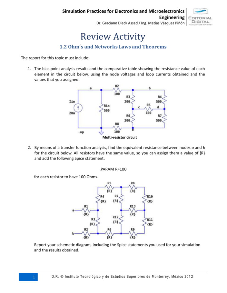
1. The bias point analysis results and the comparative table showing the resistance value of each
element in the circuit below, using the node voltages and loop currents obtained and the
values that you assigned.
Multi-resistor circuit
2. By means of a transfer function analysis, find the equivalent resistance between nodes a and b
for the circuit below. All resistors have the same value, so you can assign them a value of {R}
and add the following Spice statement:
.PARAM R=100
for each resistor to have 100 Ohms.
Report your schematic diagram, including the Spice statements you used for your simulation
and the results obtained.
1
D . R . © I n s t i tu t o T e c no l ó g ic o y d e E s t u d i o s S u p er i o re s d e M o n te rr e y , M é x i c o 2 0 1 2
Simulation Practices for Electronics and Microelectronics
Engineering
Dr. Graciano Dieck Assad / Ing. Matías Vázquez Piñón
3. Demonstrate by a hand-calculation that both, the KVL and the KCL, are fulfilled on each loop
and each node of the circuit depicted in Figure A. Also show the results of using the .measure
directive to automatically perform such calculations.
Spice Deck Version
*01.Ohm_and_Kirchhoff.asc
R1 a 0 500
R2 b a 100
R7 d 0 100
R3 c b 200
R5 d c 200
R4 c b 500
R6 d c 500
Iin 0 a 20m
.op
Schematic Version
.backanno
.end
Figure A. Voltage signs and current directions of the resistors
4. For the circuit below show your bias point analysis for both, the large and the Thevenin
equivalent circuits. Demonstrate that your results are correct with the corresponding
mathematical procedure in paper.
Spice Deck Version
*02.Thevenin.asc
V1 in 0 10
R1 a in 1k
R2 0 a 1k
R3 a out 2k
RL out 0 1k
.op
.backanno
Schematic Version
.end
Figure B. Circuit to be represented by its Thevenin equivalent
2
D . R . © I n s t i tu t o T e c no l ó g ic o y d e E s t u d i o s S u p er i o re s d e M o n te rr e y , M é x i c o 2 0 1 2
Simulation Practices for Electronics and Microelectronics
Engineering
Dr. Graciano Dieck Assad / Ing. Matías Vázquez Piñón
5. As an extension of the Thevenin's theorem, you can also represent a circuit by its equivalent
Norton's theorem that uses a current source, instead of a voltage source. As in the Thevenin's
theorem, this also applies for reactive circuits using the equivalent output impedance. Find
the Norton equivalent of the circuit in Figure B. This time, instead of an open circuit, you will
substitute the load resistor for a short circuit; the current through it will be the value of the
equivalent current source. The output resistance is the same than the Thevenin's equivalent
circuit, but this time it is also equivalent with the current source. Demonstrate that your
results are correct with the corresponding mathematical procedure in paper.
6. For the maximum power transfer demonstration, show the obtained power plot of the load
resistor RL with the resistance value for the maximum power transfer on the curve.
Demonstrate that your results are correct through the corresponding mathematical procedure
in paper.
7. For the principle of linearity demonstration, show the behavior of the relationship between
the voltage across and the current through resistor R1. Does the resistance value obtained
match the assigned in the capture of the circuit?
8. Use the circuit below to demonstrate the Superposition theorem through a Spice simulation:
You can remove any of the voltage sources by giving it a value of zero volts or by replacing it
for a short circuit. First, do this with one of the voltage sources. Then get the loop currents
and node voltages using a bias point analysis. Restore the voltage source and replace the
second in the same way. Lastly, perform a new bias point analysis with the two voltage sources
in place. Is the Superposition theorem fulfilled? Compare, by hand-calculation, your
simulation results with the mathematical procedure results.
3
D . R . © I n s t i tu t o T e c no l ó g ic o y d e E s t u d i o s S u p er i o re s d e M o n te rr e y , M é x i c o 2 0 1 2