Polynomial Curve of Best Fit
Assume that we have collected a set of n data points S = {(x1, y1), (x2, y2), …, (xn, yn)} from an
experiment or from measuring some physical situation. We can plot the data (often called a scatter
plot) but usually the points will not fall on a single straight line. Previously we used linear interpolation
to connect all the points. We saw that the result can be “spiky” and the pieces can have different
slopes. An alternative procedure is to try to determine one line which comes closest to all the points,
but need not go through (interpolate) any of the points. The line in this case is called the line of best
fit to the data. (Note that this idea is very different from interpolation which requires we go through all
of the points.)
Here we discuss a way to determine the line of best fit graphically and algebraically within MATLAB.
We describe how the equation of the line of best fit is computed, but omit the details. In addition we
show how to determine a quadratic of best fit when the data seems to have a parabolic shape.
We used the following example previously when we discussed linear interpolation. First we use
MATAB to approximate and determine the line of best fit and then discuss and compare quadratic fits.
(There are cubic fits, quartic fits, quantic fits, and in general polynomial fits of degree n.)
Example: The following is a set temperature measurements taken from the cylinder head of a new
engine that is being tested for possible use in a race car. (Source: D. Etter, Engineering Problem
Solving in MATLAB)
Time, t
0 1 2 3 4 5
Temperature, ºF 0 20 60 68 77 110
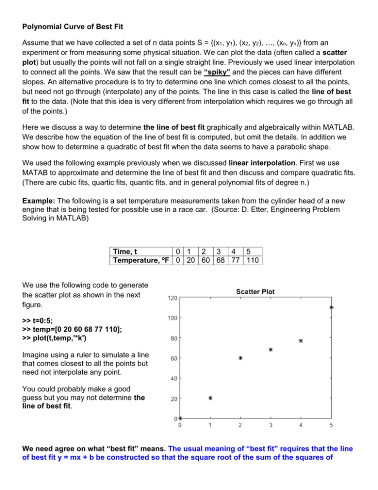
We use the following code to generate
the scatter plot as shown in the next
figure.
>> t=0:5;
>> temp=[0 20 60 68 77 110];
>> plot(t,temp,'*k')
Imagine using a ruler to simulate a line
that comes closest to all the points but
need not interpolate any point.
You could probably make a good
guess but you may not determine the
line of best fit.
We need agree on what “best fit” means. The usual meaning of “best fit” requires that the line
of best fit y = mx + b be constructed so that the square root of the sum of the squares of
vertical distances to the data points to the line is minimized. Yes, this is a max-min computation.
As such it requires the use of (partial) derivatives and the solution of a set of equations. We will use
MATLAB to perform these computations.
For now let’s see how we can approximate the line of best using an interactive MATLAB routine
called lsqgame. (The line of best fit is often referred to as least squares line.)
In this interactive 'game' you get two guesses for the least squares line by using the mouse to select
two points that are then connected to generate your approximate least squares line. Here is an
example of the graphs generated in lsqgame for the time-temperature data.
The routine permits a second try as shown next.
The line of best fit can be
computed within lsqgame
as shown in the next
figure. Note that both blue
and magenta lines were rather good approximations.
MATLAB provides an easy method for computing the equation and graphing the line of best fit once
you have plotted the scatterplot. Here is our scatter plot for the example and the code that generated
it. Read the directions on the graph.
>> t=0:5;
>> temp=[0 20 60 68 77 110];
>> plot(t,temp,'*k') %Making the scatter plot
See the next graph.
If you want to see an equation of the line
of best fit click on the arrow at the bottom
of the Basic Fitting drop down menu. See
below.
If the scatter plot seems to indicate that a curve would produce a
better model to the data we have a variety of options. The one we
discuss here is the quadratic of best fit or a quadratic least
squares fit. There is another “game” we can use to get a feel for
creating the quadratic; of course the MATLAB file is quadgame and
is played the same way lsqgame is played. Again MATLAB has an
easy way to compute the corresponding equation of the parabola of best fit and graph it.
Example: Use the following code to
create a scatter plot of the data in
the following table. The figure
shows both a quadratic and a linear
least squares fit to the data. We
used the basic fitting drop down
menu obtained by clicking on tools.
In addition, the equations for each
least squares fit are shown.
(Source: Hanselmandand Littlefield,
Mastering MATLAB, 2012.)
>> x=0:.1:1;
>> y=[-0.447 1.978 3.28 6.16 7.08 7.34 7.66 9.56 9.48 9.30 11.2];
>> plot(x,y,'*k')
>> title('Quadratic and Linear Least Squares')
Inspect the Basic Fitting menu; particularly, the boxes that are
checked. This indicates how the graph was obtained.
As we indicated previously, “best fit” requires that the
polynomial (linear, quadratic, cubic, etc.) of best fit is
constructed so that the square root of the sum of the squares of
vertical distances from the curve of best fit to the data points is
minimized. The quantity “square root of the sum of the
squares of vertical distances” is called the norm of the
residual. If you look at the menu from Basic Fitting clicking the
arrow at the bottom will give the equation of the curve of best fit
and display the residual. For our example we get that the norm
of the residual of the quadratic fit is smaller than the norm of
linear fit.
If we think of the norm of the residual as an “error measure”, then the quadratic is a “better” fit to the
data.
Will this always be the case? Explain. (Hint: think of the minimization process for the quadratic fit
as search over all polynomials of degree 2 or less.)
Could you find a best fit of a polynomial of degree n so that the norm of the residual is zero?
Explain.
Warning: Least squares line fit or quadratics are not guaranteed to produce good
approximations for all data sets.