Keily et al, Supplementary Information
Model Construction
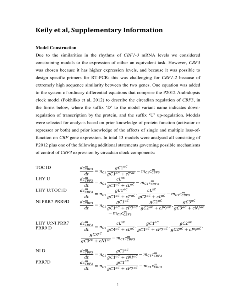
Due to the similarities in the rhythms of CBF1-3 mRNA levels we considered
constraining models to the expression of either an equivalent task. However, CBF3
was chosen because it has higher expression levels, and because it was possible to
design specific primers for RT-PCR: this was challenging for CBF1-2 because of
extremely high sequence similarity between the two genes. One equation was added
to the system of ordinary differential equations that comprise the P2012 Arabidopsis
clock model (Pokhilko et al, 2012) to describe the circadian regulation of CBF3, in
the forms below, where the suffix ‘D’ to the model variant name indicates downregulation of transcription by the protein, and the suffix ‘U’ up-regulation. Models
were selected for analysis based on prior knowledge of protein function (activator or
repressor or both) and prior knowledge of the affects of single and multiple loss-offunction on CBF gene expression. In total 13 models were analysed all consisting of
P2012 plus one of the following additional statements governing possible mechanisms
of control of CBF3 expression by circadian clock components:
TOC1D
LHY U
LHY U:TOC1D
NI PRR7 PRR9D
𝑚
𝑑𝑐𝐶𝐵𝐹3
𝑑𝑡
𝑚
𝑑𝑐𝐶𝐵𝐹3
𝑑𝑡
𝑚
𝑑𝑐𝐶𝐵𝐹3
𝑑𝑡
𝑚
𝑑𝑐𝐶𝐵𝐹3
𝑑𝑡
𝑔𝐶1𝑎𝐶
𝑚
= 𝑛𝐶1
− 𝑚𝐶1 𝑐𝐶𝐵𝐹3
𝑎𝐶
𝑎𝐶
𝑔𝐶1 + 𝑐𝑇
𝑐𝐿𝑎𝐶
𝑚
= 𝑛𝐶1
− 𝑚𝐶1 𝑐𝐶𝐵𝐹3
𝑔𝐶1𝑎𝐶 + 𝑐𝐿𝑎𝐶
𝑔𝐶1𝑎𝐶
𝑐𝐿𝑎𝐶
𝑚
= 𝑛𝐶1
.
− 𝑚𝐶1 𝑐𝐶𝐵𝐹3
𝑔𝐶1𝑎𝐶 + 𝑐𝑇 𝑎𝐶 𝑔𝐶2𝑎𝐶 + 𝑐𝐿𝑎𝐶
𝑔𝐶1𝑎𝐶
𝑔𝐶2𝑎𝐶
𝑔𝐶3𝑎𝐶
= 𝑛𝐶1
.
.
𝑔𝐶1𝑎𝐶 + 𝑐𝑃7𝑎𝐶 𝑔𝐶2𝑎𝐶 + 𝑐𝑃9𝑎𝐶 𝑔𝐶3𝑎𝐶 + 𝑐𝑁𝐼𝑎𝐶
𝑚
− 𝑚𝐶1 𝑐𝐶𝐵𝐹3
LHY U:NI PRR7
PRR9 D
𝑚
𝑑𝑐𝐶𝐵𝐹3
𝑐𝐿𝑎𝐶
𝑔𝐶1𝑎𝐶
𝑔𝐶2𝑎𝐶
= 𝑛𝐶1
.
.
.
𝑑𝑡
𝑔𝐶4𝑎𝐶 + 𝑐𝐿𝑎𝐶 𝑔𝐶1𝑎𝐶 + 𝑐𝑃7𝑎𝐶 𝑔𝐶2𝑎𝐶 + 𝑐𝑃9𝑎𝐶
𝑔𝐶3𝑐𝐶
𝑚
− 𝑚𝐶1 𝑐𝐶𝐵𝐹3
𝑔𝐶3𝑐𝐶 + 𝑐𝑁𝐼𝑐𝐶
NI D
𝑚
𝑑𝑐𝐶𝐵𝐹3
𝑔𝐶1𝑎𝐶
𝑚
= 𝑛𝐶1
− 𝑚𝐶1 𝑐𝐶𝐵𝐹3
𝑑𝑡
𝑔𝐶1𝑎𝐶 + 𝑐𝑁𝐼𝑎𝐶
𝑚
𝑑𝑐𝐶𝐵𝐹3
𝑔𝐶1𝑎𝐶
𝑚
= 𝑛𝐶1
− 𝑚𝐶1 𝑐𝐶𝐵𝐹3
𝑑𝑡
𝑔𝐶1𝑎𝐶 + 𝑐𝑃7𝑎𝐶
PRR7D
1
PRR9 D
EC D
EC U
EC TOC1 D:LHY U
EC D:LHY U
EC D:TOC1U
𝑚
𝑑𝑐𝐶𝐵𝐹3
𝑑𝑡
𝑚
𝑑𝑐𝐶𝐵𝐹3
𝑑𝑡
𝑚
𝑑𝑐𝐶𝐵𝐹3
𝑑𝑡
𝑚
𝑑𝑐𝐶𝐵𝐹3
𝑑𝑡
𝑚
𝑑𝑐𝐶𝐵𝐹3
𝑑𝑡
𝑚
𝑑𝑐𝐶𝐵𝐹3
𝑑𝑡
𝑔𝐶1𝑎𝐶
𝑚
= 𝑛𝐶1
− 𝑚𝐶1 𝑐𝐶𝐵𝐹3
𝑎𝐶
𝑎𝐶
𝑔𝐶1 + 𝑐𝑃9
𝑔𝐶1𝑎𝐶
𝑚
= 𝑛𝐶1
− 𝑚𝐶1 𝑐𝐶𝐵𝐹3
𝑎𝐶
𝑎𝐶
𝑔𝐶1 + 𝑐𝐸𝐶
𝑐𝐿𝑎𝐶
𝑚
= 𝑛𝐶1
− 𝑚𝐶1 𝑐𝐶𝐵𝐹3
𝑔𝐶1𝑎𝐶 + 𝐸𝐶
𝑐𝐿𝑎𝐶
𝑔𝐶1𝑎𝐶
𝑔𝐶2𝑎𝐶
= 𝑛𝐶1
.
.
𝑔𝐶4𝑎𝐶 + 𝑐𝐿𝑎𝐶 𝑔𝐶1𝑎𝐶 + 𝑐𝑇 𝑎𝐶 𝑔𝐶2𝑎𝐶 + 𝑐𝐸𝐶 𝑎𝐶
𝑚
− 𝑚𝐶1 𝑐𝐶𝐵𝐹3
𝑔𝐶1𝑎𝐶
𝑐𝐿𝑎𝐶
𝑚
= 𝑛𝐶1
.
− 𝑚𝐶1 𝑐𝐶𝐵𝐹3
𝑎𝐶
𝑎𝐶
𝑎𝐶
𝑎𝐶
𝑔𝐶1 + 𝑐𝐸𝐶
𝑔𝐶2 + 𝑐𝐿
𝑔𝐶1𝑎𝐶
𝑔𝐶2𝑎𝐶
𝑚
= 𝑛𝐶1
.
− 𝑚𝐶1 𝑐𝐶𝐵𝐹3
𝑔𝐶1𝑎𝐶 + 𝑐𝐸𝐶 𝑎𝐶 𝑔𝐶2𝑎𝐶 + 𝑐𝑇 𝑎𝐶
𝑚
Wherein 𝑐𝐶𝐵𝐹3
is the concentration of CBF3 mRNA; T the concentration of TOC1
protein, L the concentration of LHY protein, P7 the concentration of PRR7 protein,
P9 the concentration of PRR9 protein, NI the concentration of NI protein, and EC the
concentration of the Evening Complex. The parameters gC1-gC4 are MichaelisMenten constants, parameter aC Hill coefficients which were fixed to 2 (for
explanation see Pokhilko et al., 2012), nC1 and mC1 the rate constants for mRNA
synthesis and degradation respectively.
The model was optimised by comparing CBF3 mRNA data from 12L:12D diurnal
cycles (diurnal.mocklerlab.org/; Mockler et al, 2007; Figure 2) to simulated rhythms
using a parallel genetic algorithm (PGA) in the model optimisation framework, SBSI
Visual (http://www.sbsi.ed.ac.uk/). Parameter values for the P2012 ODEs were fixed
at their published values, and values of new parameters for each model are shown in
Supplementary Table 1. Maximum parameter values were set to 5: for higher values
the potential for variation in variable concentrations to affect simulated CBF3 gene
expression tends to zero, and are therefore not useful for the simulation of these
biological systems. CBF3 mRNA shows peak 8 hours after dawn in this dataset, and
low and invariant expression at other time-points. This background expression was
not significantly different to zero and was thus the lowest expression value for CBF3
expression in each time-series was assumed to be zero and other data-points
normalised accordingly. Use of microarray rather than RT-PCR data was considered
central to the aims of the project, as success opens the door to understanding the
control of multiple circadian outputs for which microarray data are available,
2
approximately 1/3 of the genome (Harmer et al, 2000). Model equations were solved
and simulated using the differential equation solver CVODES (Hindmarsh et al, 2005;
Serban and Hindmarsh, 2005). Parallel genetic algorithms converge to find a
parameter set where the error between the simulation and data reaches a minimum
(Muhlenbein et al, 1991). In our optimisation process, we set the target minimum
error to be 0.01. This minimum, though, could be a local minimum in the parameter
space and not the global minima. Studies have discovered that ‘sloppy’ parameters,
that are not necessarily the global minima of parameter space, lead to systems that
produce the correct dynamics in a number of conditions (Brown et al, 2004).
Simulated annealing methods attempt to find global minima but at a greater
computational cost compared to parallel genetic algorithms. Studies have shown
annealing procedures are only slightly better at finding global minima compared to
genetic algorithms (Laskey et al, 2003). The PGA method used here was found to take
O(102) iterations to converge to the fixed cost target of 0.01, compared to O(105)
iterations for simulated annealing.
Model Selection
In this study we have used model selection techniques to assess the capability of
mathematical models to describe the experimental data obtained for an output of the
Arabidopsis circadian clock. Model selection techniques provide objective, numerical
metrics to balance competing priorities of model construction. The need for a model
to describe data accurately must be weighed against the complexity of the model
(Frequentist approach) that is determined by the number of parameters in the model,
or the variability associated with the model (Bayesian approach) that arises from the
uncertainty in the values of parameters (Akaike, 1974; Burnham and Anderson, 2004;
Friel and Pettitt, 2008; Vyshemirsky and Girolami, 2008). A models accuracy and fit
to the data can be improved by increasing the number of parameters. However, due to
the overall increase in the uncertainty of the parameter values in a model with added
parameters, the model loses its predictive power. The results of model selection
analysis help to determine whether a model overfits the data as a consequence of
increased complexity.
3
All model selection techniques are based on the calculation of likelihood probabilities,
where the higher the probability, the more likely the model is able to describe the
relevant experimental data (Akaike, 1974; Burnham and Anderson, 29004; Friel and
Pettitt, 2008; Vyshemirsky and Girolami, 2008). Burnham & Anderson (2004) discuss
a number of philosophies and pitfalls in using such techniques. Here, we describe the
calculation of the corrected Akaike Information Criterion (AICc) used in this study
and attempt to build on this work to offer a similar measure that takes into account the
inherent uncertainty in model parameter values.
In the following sections we will use the following general notation: in j=1,…,D
datasets there will be i=1,…,m datapoints, ni( j ) , evaluated at certain timepoints ti; M
denotes a model simulation from a model of k parameters that takes the values Mi =
M(ti).
Calculation of AICc
The Akaike Information Criterion (AIC) was first developed in the 1970’s to
approximate the Kullback-Leiber (K-L) divergence (Akaike, 1974). For our case, the
K-L divergence is related to the distance found between data and model simulations
which we are looking to minimize. Interestingly, references point out that the K-L
divergence is related to Boltzmann’s measure of entropy that is regularly used in
information theory (Burnham and Anderson, 2004, Vedral, 2012). The AIC is
calculated as ([1]):
AIC  2 log(LMLE )  2k ,
(1)
where LMLE is the maximum likelihood estimate of the likelihood function. Hurvich &
Tsai (1989) showed that the AIC provided a rather poor approximation of the K-L
divergence when the ratio of datapoints to parameters was large (Burnham and
Anderson, 2004; Hurvich and Tsai, 2005). However, the AICc proved to be a more
accurate unbiased estimator of the K-L distance and is calculated as:
4
AICc  2 log(LMLE ) 
2q(k  1)
.
qk 2
(2)
where q is the total number of datapoints used in the analysis, ie. q  Dm . The second
term of (2) always has to be positive so that the first term is correctly ‘penalised’ by
the number of parameters in the model, i.e. q  k  2 .
In (1) and (2) we have shown the formulations of AIC and AICc featuring the
likelihood probability. As pointed out by Burnham & Anderson (2004), these results
can be reduced in the special case where we assume the differences between a
datapoint from dataset D and the model simulation at the same time follow a normal
distribution. Hence,
ni( D )  M i ~ N (0, 2 ) ,
m
where  2 
 (n
i 1
( D)
i
(3)
 M i )2
m
. This can be proven by using the central limit theorem
with a very large number of datapoints ( m   ).
Using this assumption, the first term of the AIC and AICc reduces to
 2log(LMLE )  mlog( 2 ) .
(4)
Thus, the AICc used in this study is based on
D
AICc   m( j ) log( (2j ) ) 
j 1
2q(k  1)
,
qk 2
(5)
where m(j) is the number of datapoints in dataset j.
Ensuring q > k+2 using circadian data
5
As mentioned in the previous section, for the AICc analysis to accurately penalise a
model by its complexity (or the number of parameters), then the number of datapoints
used in the analysis has to be greater than the number of parameters add two. Since
we are not comparing different models of the circadian clock, the analysis specifically
requires data of our chosen clock output, CBF3, to determine which model is
preferable. Therefore, since the circadian clock model itself features 109 parameters,
we require either a very large single dataset for our output or numerous smaller data
sets to ensure that q>k+2 is satisfied. However, genes with circadian regulation
should have a similar level of expression at the same time of day, or point of the limit
cycle, for several days/cycles. This means we can concatenate simulations and data
from one cycle such that n ( j ) (ti )  n ( j ) (ti  24(d  1)) , where d is the number of whole
days, to ensure that the number of data points is suitably large. This means that we
can take a dataset that describes 1 day to describe 3 days by repeating the dataset 3
times. For example, if we have data at t=0,4,8,12,16,20,24 with n(0)=n(24) then we
count the points in t=[0,20] three times to create three limit cycles and the t=24 once
as the final timepoint of the 3 days. Since the model simulates circadian gene
expression on a limit cycle, the simulations at the respective timepoints will also be
the same in day 1 as day 3. As we have concatenated the data for both AICc and
AICcU, the later discussions comparing results from the two methods are independent
of the data repetition used here to ensure q>k+2. Figure S1 shows an example of a
model and dataset in 12L:12D cycles. Hence, we can adapt the AICc to ensure that
the penalty term is always positive:
D
D
AICc  d  (m( j )  1) log( (2j )
j 1
D
2
t  24 )   log( ( j )
j 1
t 24
)
2(d  (m( j )  1)  D)( k  1)
(6)
j 1
D
d  (m( j )  1)  D  k  2
j 1
D
where d is the number of days required to ensure that d  (m( j )  1)  D  k  2 and
j 1
log( (2j )
t i
) is the value of log( (2j ) ) evaluated for the t=i timepoint. The third term
of this equation shall be referred to as the ‘penalty’ term
6
D
Z
2(d  (m( j )  1)  D)(k  1)
j 1
D
d  (m( j )  1)  D  k  2
.
j 1
Akaike Weights
Whereas AICc scores can generally take on a wide range of values, Akaike Weights
use the AICc scores to provide a probability measure for a model variant from the set
of models (Burnham and Anderson, 2004). Thus, the higher the probability for a
given model, M, the more likely it is that M fits the data without overfitting the data.
This provides us with our measure of deciding which model variant from our set is
favoured. They are calculated as
p( M ) 
exp{ s / 2}
 exp{ r / 2}
(7)
r
where  s  AICcs  AICcmin is the relative AICc score and AICcmin is the minimum
value of AICc from the set of r models that corresponds to the ‘best’ model
([1],[2],[5]). Values of s  10 imply that a model does not have any statistical
support. If a model has a value of s  10 then the model has statistical support, with
the significance increasing as  s  0 (Burnham and Anderson, 2004). These values
thus show how much more likely one model is favoured compared to another.
Model Uncertainty in AICc (AICcU)
The AICc is generally seen as a Frequentist measure by statisticians as it supposes
that the value of the parameters, kl, are fixed. In comparison, Bayesian statistical
inference includes the uncertainty associated with parameter values of a model. The
reason for this is that the important properties of a specific model are expected to be
robust such that they are maintained over a range of parameter values (for example
see Song et al, 2012; Pokhilko et al, 2012). Hence, the ‘true’ parameter value lies
somewhere within this range but we are uncertain of the exact value (see
7
Supplementary Figure 1). To characterise this uncertainty, Bayesian inference looks
to calculate the posterior distribution such that
Posterior  Prior x Likelihood
where the prior distribution is the probability distribution of the model/parameter
variability and the likelihood is the same as that discussed previously.
As outlined in Burnham & Anderson (2004), Bayesian approaches to AIC measures
(for example, the Bayesian/Schwarz Information Criterion; B/SIC) assume that the
‘true’ model is one of the variants found in our set of possible models, which we
cannot assume here. However, since the AICc and BIC both have a close relationship
to likelihood probabilities, we rationalised that if we could approximate the
uncertainty in parameter values through a prior probability, then we could include a
further term to the calculation of AICc scores. In doing this, the new AICc scores
(termed AICcU below) would not only take into account the number of parameters
used in the model, but also the uncertainty in their parameter values.
Since the calculation of prior distributions can become quite complicated (we
evaluated methods such as Thermodynamic Integration found in Friel and Pettitt
(2008) and Vyshemirsky, and Girolami (2008)), we made the assumption that the
simplest model to describe the data was a sine curve due to the circadian rhythm of
the output gene expression. In our example for this study, the circadian regulation of
CBF3 mRNA was analysed. As our models were optimised to data from 12(hours)
L:12(hours) D cycles, we ensured that the peak of the sinewave matched the peak of
the data from the same conditions (at ZT8; see Figure S1). We then assumed, as with
the difference between the datapoints and model simulations earlier, that the
differences between the models in 12L:12D cycles and our prior model followed a
normal distribution. Hence, our prior distribution is defined as
M ~ N (  , 2 )
(8)
8
where  is the value of the sinewave at ti and  2 is the variance calculated in the
same manner as  2 (see later discussion). Therefore, the full AICcU is
m
AICcU  AICc  log( 2 ) 
 (M
i 1
i
(9)
  )2
2
 AICcU
where AICc is calculated from (6). From (9), when  2   , AICc
since the
s
s
last term will tend to zero and the logarithmic term will become a constant that will
disappear when  s values are calculated.
Results of Analysis
The results for the AICc analysis are included in the main text (see Table 1). Here we
will summarise and discuss the results of the AICc and AICcU analysis, paying
particular attention to the values of the number of data cycles, d, and the variance in
model simulations due to perturbed parameter values,  2 , used.
Does the prior distribution change conclusions drawn from AICc?
Supplementary Table 2 shows the AICcU scores using a value of d = 4 and allowing
 2 to be calculated in the same way as  2 for each model. Comparing these results to
Table 1 shows that the same model (EC TOC1 D: LHY U) is favoured by using the
AICcU analysis. To test whether this result was a consequence of maintaining the use
of the Z penalty term in the AICcU analysis, we carried out the analysis again without
penalising models for complexity. From Supplementary Table 2, we observed that
removing Z did not affect which model was selected as best from the set, leading to
stronger support for EC TOC1 D: LHY U as seen by the Δs values. This suggests that
the same result can be achieved by penalising a model for the number of parameters
in the system or by calculating a prior distribution for parameter uncertainty. However,
due to the increased support of EC TOC1 D: LHY U this result also suggests that
prior distributions may not penalise model complexity stringently enough, allowing
one of the most complex models to dominate the result. Due to these observations
9
made from Supplementary table 2, we based our results on the AICc analysis (Table 1,
main text) that did not require prior information on model structure and had a stronger
penalty for model complexity.
Does the value of  2 affect the results?
Over a range of  2 values, the most probable model from the AICcU analysis did not
change and EC TOC1 D: LHY U was always selected as the most probable model.
However, the likelihood of other models relative to this favoured model did change
over the range of  2 . Supplementary Figure 2 shows how the Δs of EC TOC1 D and
EC D: LHY U - the two ‘closest’ models to EC TOC1 D: LHY U - change with  2
for d = 4. From the figure, we observed that the conclusions drawn from the analysis
were unaffected by the value of  2 such that Δs > 0 for all  2 implying that EC
TOC1 D: LHY U would always be selected as the best model from the set. However,
this may be a special case, and the value of  2 may play a larger role in determining
which model was most suitable if the analysis had been run on a set of models where
the differences in accuracy to data were smaller. In particular, values of Δs seem to
change more dramatically as  2  0 .
How does the value of d affect results?
As the total number of datapoints that was being used in the analysis was
D
 (m
j 1
( j)
 1)  D  98 and the largest model contained k = 130 parameters the
minimum value of d that could be used was d = 2 to ensure that
D
d  (m( j )  1)  D  k  2 . From Supplementary Figure 3a, we observed that when d <
j 1
3, EC D is selected as the suitable model from the set using AICc. This model
contains CBF3 regulation solely through repression from the evening complex (EC)
of the circadian clock. When d ≥ 3, the analysis concludes that EC TOC1 D: LHY U
is the most appropriate system for CBF3 regulation. The increase in d leads to an
increase in the number of data points considered in the analysis (see above), which in
turn has been shown to improve the accuracy of AICc scores in comparison to the true
10
Kullback-Leiber divergence (Hurvich and Tsai, 1989). The results quoted in Table 1
and Supplementary Table 2 are for the case where d = 4.
The reason for the change in results with the change in d can be observed from
Supplementary Figure 3 where the difference between Z-values of EC TOC1 D: LHY
U (k=128) and EC D (k=124) has been calculated. This shows that EC TOC1 D: LHY
U is penalised more than EC D regardless of d. However, as d increases, the increased
penalty for EC TOC1 D: LHY U decreases relative to the penalty for EC D, i.e. the
difference between the two terms decreases. This means that the difference in the
AICc values for EC TOC1 D: LHY U and EC D would become more dependent on
the accuracy of the simulations compared to the data. Since EC TOC1 D: LHY U is
D
more accurate than EC D (  m( j ) log( (2j ) )  D  320.4  290.7 , where the lower
j 1
value implies accuracy), this difference would be amplified as d increases,
overcoming the difference in penalty terms.
Model analysis
To simulate circadian clock null mutants the corresponding protein levels were fixed
at zero. Gating by low temperature was simulated by assuming a 5-fold increase in
either LHY nuclear protein or CBF mRNA levels as indicated. Simulations were
compared to data presented in Figure 2A from Fowler et al, (2005). Northern blot
image was imported in Photoshop (Adobe systems) and maximum CBF expression
after cold at each time point calculated using the histogram function, and are
presented in arbitrary units. Simulation outputs were scaled such that the maximum
values of CBF expression were equivalent to the maximum value in the observed data.
Although the observed data was obtained by hybridisation to a CBF2 probe,
experiments elsewhere in Fowler et al, (2005) show that CBFs1-3 behave similarly. In
order to check that the performance of our model of CBF3 regulation by LHY, TOC1
and EC is robust to parameter variation we performed sensitivity analysis using
COPASI, analysing the fold change in CBF3 expression at 4 hour intervals across one
light dark cycle with a delta factor of 0.001 and a delta minimum of 1e-12.
(Supplementary Table 3). This showed that parameters that govern the relationship of
LHY, TOC1 and EC with CBF3 mRNA levels were among the least sensitive in the
model, the most sensitive being the degradation rate of CBF3 mRNA, and parameters
11
governing the light sensitivity of the clock mechanism. That an appropriate CBF3
degradation rate is essential for the fast fall in CBF levels after transcriptional
inhibition is not surpising, and the model was only sensitive to CBF3 degradation rate
in the hours following the period of peak expression. We therefore conclude that the
core properties of our model are not manifest with a small unique parameter range,
and that the model is robust to local variation of new parameter values, with the
exception of CBF3 degradation rates, which must be fast.
Supplementary References
Akaike H. (1974) A new look at the statistical model identification. IEEE
Transactions on Automatic Control 19: 716-723
Burnham KP, Anderson DR. (2004) Multimodel inference: Understanding AIC and
BIC in model selection. Sociological Methods Research 33: 261-304.
Dong MA, Farre I. and Thomashow MF. (2011) CIRCADIAN CLOCKASSOCIATED 1 and LATE ELONGATED HYPOCOTYL regulate expression of
the C-REPEAT BINDING FACTOR (CBF) pathway in Arabidopsis. PNAS 108:
7241-7246
Fowler SG, Cook D, Thomashow MF. (2005) Low temperature induction of
Arabidopsis CBF1, 2, and 3 is gated by the circadian clock. Plant Physiol 137: 961968
Friel N, Pettitt AN. (2008) Marginal likelihood estimation via power posteriors.
Journal of the Royal Statistical Society B 70: 589-607
Harmer SL, Hogenesch JB, Straume M, Chang HS, Han B, Zhu T, Wang X,
Kreps JA, Kay SA. (2000) Orchestrated transcription of key pathways in
Arabidopsis by the circadian clock. Science 290: 2110-2113
Hindmarsh AC, Brown PN, Grant KE, Lee SL, Serban R. (2005) SUNDIALS:
Suite of nonlinear and differential/algebraic equation solvers. ACM Transactions on
Mathematical Software 31: 363-396
Hurvich CM, Tsai CL. (1989) Regression and time series model selection in small
samples. Biometrika 76: 297-307
Laskey KB, Myers JW. (2003) Population markov chain monte carlo. Machine
Learning 50: 175-196
Mockler TC, Michael TP, Priest HD, Shen R, Sullivan CM. (2007) The
DIURNAL project: Diurnal and circadian expression profiling, model-based pattern
matching and promoter analysis. Cold Spring Harbor Symposium Quantitative
Biology 72: 353-363
12
Muhlenbein H, Schomisch M, Born J. (1991) The parallel genetic algorithm as
function optimizer. Parallel Computing 17: 619-632
Novillo F, Medina J, Salinas J. (2007) Arabidopsis CBF1 and CBF3 have a different
function than CBF2 in cold acclimation and define different gene classes in the CBF
regulon. Proc. Natl. Acad. Sci. USA, 104, 21002-21007.
Pokhilko A et al. (2012) The clock gene circuit in Arabidopsis includes a
repressilator with additional feedback loops. Molecular Systems Biology 8: 574
Serban R, Hindmarsh AC. (2005) CVODES: the sensitivity-enabled ODE solver in
SUNDIALS. Proceedings of IDETC/CIE
Song YH et al. (2012) FKF1 conveys timing information for CONSTANS
stabilization in photoperiodic flowering. Science 336: 1045-1049.
Vedral V. (2012) Decoding reality: The universe as quantum information. Oxford
University Press.
Vyshemirsky V, Girolami MA. (2008) Bayesian ranking of biochemical system
models. Bioinformatics 24: 833-839.
13
Supplementary Tables
Model
TOC1D
LHY U
LHY U TOC1 D
PRR7 PRR9 NI D
LHY U NI PRR7
PRR9 D
NI D
PRR7 D
Parameter
mC1
nC1
gC1
aC
mC1
nC1
gC1
aC
mC1
nC1
gC1
gC2
aC
mC1
nC1
gC1
gC2
gC3
aC
Value
0.2746
5.0000
0.0081
2.0000
0.2176
0.2419
0.7667
2.0000
0.2350
4.9751
0.0103
0.4754
2.0000
0.0583
0.5224
5.0000
5.0000
0.0270
2.0000
Model
PRR9 D
Parameter
mC1
nC1
gC1
aC
mC1
nC1
gC1
aC
mC1
nC1
gC1
aC
Value
5.0000
0.9475
5.0000
2.0000
2.3963
5.0000
0.0002
2.0000
0.0250
4.7871
1.9305
2.0000
LHY U EC TOC1 D
mC1
nC1
gC1
gC2
gC4
aC
1.4070
4.9967
0.0434
0.0005
0.1344
2.0000
mC1
0.2059
LHY U EC D
mC1
2.0390
nC1
gC1
gC2
gC3
gC4
aC
mC1
nC1
gC1
aC
mC1
nC1
gC1
aC
0.2608
5.0000
5.0000
5.0000
0.8186
2.0000
0.3682
0.0711
5.0000
2.0000
0.2683
0.0511
5.0000
2.0000
nC1
gC1
gC2
aC
5.0000
0.0003
0.4020
2.0000
mC1
nC1
gC1
gC2
aC
1.9056
3.9652
0.0004
0.0723
2.0000
EC D
EC U
EC TOC1 D
Supplementary Table 1. Optimised new parameter values for each of the thirteen
models.
14
Model
AICcU
TOC1D
LHY D
LHY U: TOC1↓
NI PRR7 PRR9 D
LHY U: NI PRR7 PRR9 D
NI D
PRR7 D
PRR9 D
EC D
EC U
EC TOC1 D: LHY U
EC D: LHY U
EC TOC1 D
-301.9
-234.1
-284.8
-102.6
-199.8
-26.4
-25.0
-18.1
-634.7
-141.7
-734.4
-665.9
-678.6
With Z
%
s
432.3
500.2
449.4
631.4
534.6
707.0
708.4
715.2
99.6
591.8
0.0
68.5
55.8
0%
0%
0%
0%
0%
0%
0%
0%
0%
0%
100%
0%
0%
AICcU
Without Z
%
s
-692.5
-624.7
-685.2
-503.0
-620.4
-417.0
-415.6
-408.8
-1025.3
-532.3
-1144.8
-1066.3
-1079.0
452.1
520.0
459.4
641.4
524.4
726.9
728.2
735.1
119.5
611.7
0
78.5
65.8
0%
0%
0%
0%
0%
0%
0%
0%
0%
0%
100%
0%
0%
Supplementary Table 2: AICcU analysis results. Analysis was run with and without
the penalising of the number of model parameters (2nd term in (9)). d = 4.
15
Process
parameter
0
4
8
fold-change in CBF3 expression
12
16
20
24
-7.5791
-2.9703
-0.6751
-0.4786
-0.3550
0.9452
1.4847
0.1102
-3.7692
-4.2381
-1.0835
1.0093
4.0990
0.0404
-0.0086
0.01102
0.03799
0.09762
0.8533
3.7632
0.01307
0.4296
0.4341
0.3416
0.9600
g5
-1.2378
-1.7304
-2.3497
-3.4919
-3.3917
-1.8436
-1.0352
g7
-0.0186
-3.4220
-0.1422
0.07550
0.0610
-0.0119
-0.0167
m4
1.0758
1.8731
1.8610
3.1939
3.2043
0.8864
-0.0038
m3
1.1209
3.0383
0.5239
-2.5014
-3.1836
-2.1718
0.0500
g3
0.4061
0.3210
0.9196
2.8403
3.1639
1.5340
0.0974
p3
-0.1124
0.1388
-0.8612
-2.813
-3.0431
-1.2100
0.0763
LHY inhibition by PRRs
g1
1.1323
1.9246
1.5942
2.8389
2.9078
1.5544
0.40368
binding of ELF3 to GI
p17
-1.7329
-2.6658
0.0761
1.4649
1.7247
-0.9330
-1.6330
inhibition of GI by LHY
g15
-0.7633
2.6284
0.8540
1.5771
1.6236
-0.2328
-0.7312
p28
0.65076
2.4337
0.2818
-0.1579
-0.3288
0.1850
0.5927
n2
-1.3576
-1.6208
-1.6313
-2.4036
-2.4317
-1.8960
-1.1214
p4
-1.3523
-1.6100
-1.6264
-2.3963
-2.4244
-1.8961
-1.1239
m16
1.1784
2.3782
1.2444
1.8116
1.8224
1.1574
0.5332
q1
-0.9019
-2.2764
0.2689
1.8124
1.9007
0.1975
-0.5603
g6
1.1336
0.5166
-0.4290
-2.0977
-2.2378
0.3279
0.9528
m34
0.8702
2.1391
-0.4776
0.2212
0.4955
0.8042
1.1906
m18
2.1206
-1.0163
-0.0652
-1.4907
-1.9199
0.8764
1.9680
m11
1.0535
0.4039
-0.1365
-1.9519
-2.1104
-0.2475
0.6498
m31
-0.0179
-2.1085
-0.1997
-0.2366
-0.2280
-0.0082
-0.0307
n12
-2.0156
-0.6084
0.1940
1.6947
2.0715
-0.8569
-1.8794
p11
-1.995
1.4163
0.1676
1.6329
2.0267
-0.8339
-1.8603
q2
0.01949
2.0248
-0.0260
-0.0609
-0.0434
0.0219
0.0186
gC2
2.0010
1.9368
0.4040
1.1286
1.2957
1.8726
2.0009
gC1
1.0840
1.1167
1.2208
1.7306
1.7594
1.6650
1.0844
gC4
-0.1771
-0.0379
-0.1286
-0.4256
-0.5555
-1.0514
-0.1778
degradation rate of
CBF3 mRNA
mC1
-0.6753
-0.4788
-0.9705
-3.0172
translation of COP1
N5
1.2679
5.3098
-0.4674
m1
1.9480
4.5889
m37
0.0888
m32
light induced
degradation of LHY
mRNA
affect of light on
COP1 conformation
light induced affect of
GI on EC
inhibition of toc1 by
LHY
light induced affect of
GI on EC
degradation rate of
LHYmod
light-independent
degradation of LHY
light-induced
degradation of LHY
protein
degradation of LHY
protein
nucleocytoplasmic
transport of GI
protein
rate constant for
TOC1 transcription
rate constant for
TOC1 translation
degradation of NI
mRNA
light induced LHY
transcription
inhibition of ELF4
translation by LHY
degradation of ELF4
mRNA
degradation of GI
mRNA
degradation of light
sensitive protein P
post-translational
modification of COP1
rate constant for GI
transcription
rate constant for GI
translation
light induced
translation of GI
CBF3 inhibition by EC
CBF3 inhibition by
TOC1
CBF3 activation by
LHY
Supplementary Table 3. Sensitivity heatmap fort the expression of CBF3 at the
indicated time after dawn. Values indicate the fold-change in CBF3 mRNA value
16
with respect 4 hour intervals where dawn is 0 and 24 hours. The 20 most sensitive
parameters are shown, in addition to the parameters gC2, gC1 and gC4 which govern
regulation of CBF3 by EC, TOC1 and LHY. This analysis shows that the model is
robust to variation in new parameter values, with the exception of the CBF3 mRNA
degradation rate constant. Fast degradation is necessary to produce the sharp
waveform observed. Increases in expression are shown in blue with –ve values,
decreases in orange with +ve values.
17
Position
in Locus
Sequence
Figure 5B
A
CBF1 5’
AAAAGTCTTGCAACTTAACACTCTCA
A
CBF1 5’
TGTTCGTGGCCACATATCAT
B
CBF1 5’
GACGGGTGACAATTAATGACAAT
B
CBF1 5’
ATATTGGCCGGAGGAGAGAT
C
CBF1 ORF
GGAGACAATGTTTGGGATGC
C
CBF1 ORF
CGACTATCGAATATTAGTAACTCC
D
CBF3 5’
TTTAGCAACAGAAAGCCACAAA
D
CBF3 5’
AGTGAACTGGGCTGAATTTTT
E
CBF3 5’
GTTTAAACACAGCAGGAAGTAAATTAT
E
CBF3 5’
TCGGAAGTCAAAATAAAAAGCA
F
CBF3 5’
TGAATAACGGTTACCCTACACC
F
CBF3 5’
AGTTTTATAAACTCTTTGCGCGTATGAA
G
CBF3 ORF
AATATGGCAGAAGGGATGCT
G
CBF3 ORF
ACTCCATAACGATACGTCGT
H
CBF3 3’
GATGACGACGTATCGTTATGGA
H
CBF3 3’
GGTTTTGCTGAATCGGTTGT
I
CBF25’
TGCACGATATGTGAATGGAGA
I
CBF2 5’
TCAAGGCTGTCAATCACTGAG
J
CBF2 ORF
CGACGGATGCTCATGGTCTT
J
CBF2 ORF
TCTTCATCCATATAAAACGCATCTTG
-VE control
ACT2
CGTTTCGCTTTCCTTAGTGTTA
-VE control
ACT2
AGCGAACGGATCTAGAGACTC
Supplementary Table 4. Primer sequences for chromatin Immunoprecipitation.
Positions for each primer pair are shown in Figure 5B.
18
Supplementary Figures
Figure S1: Generalised method used for comparing models. Models were fitted to
data (red dashes, squares) with the resulting example simulation (blue, triangles) in 12
hrs light (12L):12 hrs dark (12D) cycles.  2 was calculated from the difference
between the model simulations and datapoints at the specific times of the day. A prior
model was constructed using a sinewave (black line). The difference between the
models and prior model was calculated at the same timepoints as the models were
compared to the data, M    . The region around the prior model sinewave (grey
2
dashes) represents the space in which a model may lie given a perturbation to the
prior model parameters. This space is characterised by the uncertainty in parameter
values,  2 .
19
Figure S2: Effect of  2 . The AICcU analysis was carried out over a range of  2
values (d = 4). Δs values for EC TOC1 D (black line) and EC D: LHY/CCA1 U (red
line) show that there would be no change in which model was favoured over the range
of  2 values. If the lines crossed, then that would suggest that conclusions drawn
from the analysis would change at a specific value of  2 .
20
Figure S3: Effect of d. (a) The AICc analysis was carried out over a range of d ≥ 2.
When d < 3, EC D was more favoured than EC TOC1 D: LHY U. When d ≥ 3, EC
TOC1 D: LHY U was the most probable model. d = repression/ downregulation; u =
activation/ upregulation. (b) The difference between the penalty terms of EC TOC1 D:
LHY U and EC D decreases as d is increased. This was calculated by taking the value
of Z from (6) and subtracting (EC TOC1 D: LHY U – EC D).
21
Figure S4: Published CBF1 Real-time PCR primers appear to prime from CBF1
and CBF3. Chart to show CBF1 expression (using primers published in Bienewska et
al., 2008 and Dong et al., 2011) in wild type and CBF1 RNAi, cbf2 mutants and
CBF3 RNAi plants (Novillo et al., 2007). Both CBF1 and CBF3 primers detect
elevated expression in CBF3 RNAi plants.
CBF1_F
Primer
20
CBF1
60
CBF3
60
------------------------GGAGACAATGTTTGGGATGC---------------CGAAGGTGCGTTTTATATGGATGAGGAGACAATGTTTGGGATGCCGACTTTGTTGGATAA
CGAAAATGCGTTTTATATGCACGATGAGGCGATGTTTGAGATGCCGAGTTTGTTGGCTAA
***.*.*******.****
CBF1_R
Primer
24
CBF1
54
CBF3
54
-------------------GGAGTTACTAATATTCG-ATAGTCG----------------GGTGACGTGTCGCTTTGGAGTTACTAATATTCG-ATAGTCGTTTCCATTTTTGTA
GATGACGACGTATCGTTATGGAGTTATTAAAACTCAGATTATTATTTCCATTTT---******* ***:* **. **: * .
.
Figure S5: Alignment of published CBF1-specific primers with CBF1 and CBF3
cDNA sequences. Although mis-matches occur, similarity is high and may require
very specific PCR conditions to discriminate between the two transcripts. The CBF3
sequence shown is nucleotides 634-669 to 740-793 of the 908bp cDNA. The CBF3
22
RNAi construct reported by Novillo et al (2007) includes the 3’ end of CBF3 and
starts at base number 730 and therefore is not reported to include the sequence
complimentary to CBF1_F above.
23