ANVAR et al.: Multi-View Face Detection and Registration Requiring Minimal Manual Intervention
APPENDIX A
Finding Distinctive Features
The scale invariant features (SIFT) extracted from face
images will usually return a substantial number of common or not informative features in addition to the required distinctive features. Thus, it is necessary to select
only the distinctive features obtained from the discriminative parts of a face. Two hypotheses exist, either the
feature is part of a face (𝐻𝑖,𝑘 = 1) or it is from the background (𝐻𝑖,𝑘 = 0). As at this stage, we do not know where
the face is, we assume that the distinctive feature arising
from the face should be unique. Thus in order to identify
the distinctive features and discard common features, a
likelihood ratio test (A.1) is performed to all the features
extracted from both images. Those features with likelihood ratio less than one are considered as common features and are discarded.
𝛾(𝑓𝑖,𝑘 ) =
𝑃(𝐻𝑖,𝑘 = 1|Ω)
𝑃(𝐻𝑖,𝑘 = 0|Ω)
< 1,
(A. 1)
where 𝑓𝑖,𝑘 is the kth feature of the image i, γ(fi,k ) is the likelihood ratio for this feature when some independent data Ω has been seen. As 𝛾(𝑓𝑖,𝑘 ) has to be determined for all
features found in the image, we use the Bernoulli distribution in (A.2) to determine the probability that a feature
𝑓𝑖,𝑘 comes from a part of object or non-object (𝐻𝑖,𝑘 𝜖{0,1}).
𝑃(𝐻𝑖,𝑘 |𝜃) = 𝜃 𝐻𝑖,𝑘 (1 − 𝜃)1−𝐻𝑖,𝑘 ,
(A. 2)
where 𝜃 is the distribution parameter. We use the maximum likelihood estimate (MLE) to estimate the probability in (A.1) as follows: Let feature 𝑓1,𝑘 be a feature from
1
the first image 𝐼1 which compared to all 𝑁2 features (𝑓2,𝑗 ,
𝑗 = 1, … , 𝑁2 ) in the second image 𝐼2 . If this feature is a distinctive feature, it should be unique and the occurrence of
it in the other part of the image (both face and background) would be very limited. Ideally, there would only
be one such feature and for symmetrical parts, only two
features can be found. Thus, we can estimate its probabil2
ity as 𝑃(𝐻1,𝑘 = 1|Ω) = . But if this feature originates
𝑁2
from the non-distinctive part of the image, the number of
similarities found for it could be any number, 𝛼 > 2.
Thus, we can estimate its probability as 𝑃(𝐻1,𝑘 = 0|Ω) =
𝛼
. To compute the similarity number, 𝛼, of feature 𝑓1,𝑘 in
𝑁2
𝐴
the first image, its appearance descriptor (𝑓1,𝑘
) is com𝐴
pared to the appearance descriptors (𝑓2,𝑗 ) of all features in
2
A
A
the second image within a global threshold ((f1,k
-f2,j
) <
a
Thr ). This procedure is then repeated for each feature
found in the second image, which is then compared to all
the features in the first image. Finally, all common features found are removed. To estimate the suitable value
for 𝑇ℎ𝑟 𝑎 several image pairs from different databases
(FERET, CMU, and FDDB) with various poses (left, right
and frontal views) are used for evaluation. Some sample
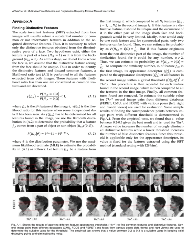
results of finding the correspondence points between image pairs with different threshold is demonstrated in
Fig.A.1. From the empirical tests, we found that a value
between 0.2-0.3 gives the best result and is used for Thr a .
A larger value increases the number of wrongly eliminated distinctive features while a lower threshold increases
the number of false distinctive features. Since this threshold is applicable only for the appearance descriptor, its
value is fixed for the features extracted using the SIFT
method (standard setting with 128 bins).
Fig. A.1. Shows the results of applying different feature appearance thresholds (𝑇ℎ𝑟 𝑎 ) to find common features and distinctive features. Several image pairs from different databases (CMU, FDDB and FERET) and faces from various poses (left, frontal and right views) are used to
determine the suitable value for the threshold. The empirical test shows that a value between 0.2 to 0.3 is a suitable value in keeping valid
distinctive points and eliminating the noise.
2
IEEE TRANSACTIONS ON PATTERN ANALYSIS AND MACHINE INTELLIGENCE,
APPENDIX B
𝑃(𝜃|𝜓)
Face Features Estimation
Let feature 𝑓𝑘 be a binary random variable that might
originate from a part of face (𝐻𝑘 = 1) or non-face (𝐻𝑘 = 0)
area. We can assign a Bernoulli distribution with parameter 𝜃 to it that determines its uncertain value as:
𝑃(𝐻𝑘 |𝜃) = 𝜃 𝐻𝑘 (1 − 𝜃)1−𝐻𝑘 ,
(𝐵. 1)
Assuming a sequence of 𝐿 independent observation of
data 𝜓 over feature 𝑓𝑘 in the training data, the likelihood
of obtaining 𝜓 is given by:
𝐿
𝑗
𝑗
𝑃(𝜓|𝜃) = ∏ 𝜃𝐻𝑘 (1 − 𝜃)𝐻𝑘 = 𝜃 𝐿𝑘 (1 − 𝜃)𝐿−𝐿𝑘 ,
(𝐵. 2)
=
1
𝛤(𝛼1 +𝛼0 ) 𝛼 −1
𝜃 𝐿𝑘 (1 − 𝜃)𝐿−𝐿𝑘
𝜃 1 (1 − 𝜃)𝛼0 −1
𝑃(𝜓)
𝛤(𝛼1 )𝛤(𝛼0 )
= 𝐵𝑒𝑡𝑎(𝜃|𝐿𝑘 + 𝛼1 , 𝐿 − 𝐿𝑘 + 𝛼0 ),
To calculate the probability of 𝑓𝑘 from a sequence of 𝐿
observation data, the uncertainty of the distribution parameter 𝜃 is considered by integrating the feature probability function over 𝜃 distribution as in (B.8). This gives
the probability that feature 𝑓𝑘 comes from a part of face
(𝐻𝑘 = 1) when a sequence of 𝐿 observation data 𝜓 over
this feature is given but the number of them is small.
𝑗=1
1
where 𝐿𝑘 is the number of time that feature 𝑓𝑘 has represented a face area in the observation data 𝜓. When 𝐿 is
large, we can estimate the distribution parameter 𝜃 using
MLE estimation as:
𝜃̂ 𝑀𝐿𝐸 = 𝑎𝑟𝑔𝑚𝑎𝑥 𝑃(𝜓|𝜃),
(𝐵. 3)
𝜃
𝛤(𝛼1 +𝛼0 ) 𝛼 −1
𝜃 1 (1 − 𝜃)𝛼0 −1 ,
𝛤(𝛼1 )𝛤(𝛼0 )
(𝐵. 4)
where α1 and α0 are hyper-parameters and is influenced
by the number of virtual face/non-face data. The gamma
function 𝛤(𝑥) is given by:
∞
𝛤(𝑥) = ∫ 𝑢 𝑥−1 𝑒 −𝑢 𝑑𝑢 ,
(𝐵. 5)
0
Considering the Bayesian rule, the posterior probability of
the distribution parameter 𝜃 can be calculated in the form
of prior probabilities as:
𝑃(𝜃|𝜓) =
𝑃(𝐻𝑘 = 1|𝜓) = ∫ 𝑃(𝐻𝑘 = 1|𝜃)𝑃(𝜃|𝜓) 𝑑𝜃
0
1
= ∫ 𝜃 𝑃(𝜃|𝜓) 𝑑𝜃
0
1
= ∫ 𝜃𝐵𝑒𝑡𝑎(𝜃|𝐿𝑘 + 𝛼1 , 𝐿 − 𝐿𝑘 + 𝛼0 ) 𝑑𝜃
0
However, if 𝐿 is small, the MLE will produce a bias outcome and there is also the sparse data problem. Since we
know that the number of false correspondences will be
low, we used Bayesian approach and considering another
uncertainty on the distribution parameter 𝜃. Thus, we
used a Beta probability distribution with prior probability
as:
𝑃(𝜃|𝛼1 , 𝛼0 ) =
(𝐵. 7)
𝑃(𝜓|𝜃)𝑃(𝜃|𝛼1 , 𝛼0 )
,
𝑃(𝜓)
(𝐵. 6)
Substituting (B.2) and (B.4) into (B.6) yields another Beta
distribution with new hyper-parameters:
=
𝐿𝑘 + 𝛼1
,
𝐿 + 𝛼1 + 𝛼0
(B. 8)