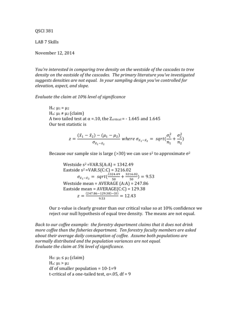
QSCI 381
LAB 7 Skills
November 12, 2014
You’re interested in comparing tree density on the westside of the cascades to tree
density on the eastside of the cascades. The primary literature you’ve investigated
suggests densities are not equal. In your sampling design you’ve controlled for
elevation, aspect, and slope.
Evaluate the claim at 10% level of significance
Ho: µ1 = µ2
Ha: µ1 ≠ µ2 (claim)
A two tailed test at α =.10, the Zcritical = - 1.645 and 1.645
Our test statistic is
𝑧=
(𝑥̅1 − 𝑥̅2 ) − (𝜇1 − 𝜇2 )
𝜎12 𝜎22
𝑤ℎ𝑒𝑟𝑒 𝜎𝑥̅ 1 −𝑥̅2 = 𝑠𝑞𝑟𝑡( + )
𝜎𝑥̅ 1 −𝑥̅2
𝑛1 𝑛2
Because our sample size is large (>30) we can use s2 to approximate σ2
Westside s2 =VAR.S(A:A) = 1342.49
Eastside s2 =VAR.S(C:C) = 3216.02
1324.49
3216.02
𝜎𝑥̅ 1 −𝑥̅2 = 𝑠𝑞𝑟𝑡( 50 + 50 ) = 9.53
Westside mean = AVERAGE (A:A) = 247.86
Eastside mean = AVERAGE(C:C) = 129.38
(247.86−129.38)−(0)
𝑧=
= 12.43
9.53
Our z-value is clearly greater than our critical value so at 10% confidence we
reject our null hypothesis of equal tree density. The means are not equal.
Back to our coffee example: the forestry department claims that it does not drink
more coffee than the fisheries department. Ten forestry faculty members are asked
about their average daily consumption of coffee. Assume both populations are
normally distributed and the population variances are not equal.
Evaluate the claim at 5% level of significance.
H0: µ1 ≤ µ2 (claim)
Ha: µ1 > µ2
df of smaller population = 10-1=9
t-critical of a one-tailed test, α=.05, df = 9
=T.INV(.05, 9) = 1.833
(𝑥̅1 − 𝑥̅2 ) − (𝜇1 − 𝜇2 )
𝑠12 𝑠22
𝑡=
𝑤ℎ𝑒𝑟𝑒 𝑠𝑥̅1 −𝑥̅2 = 𝑠𝑞𝑟𝑡 ( + )
𝑠𝑥̅1 −𝑥̅2
𝑛1 𝑛2
Variance fisheries = VAR(A:A) = 1.88
Variance forestry = VAR(C:C) = 0.66
Mean fisheries = AVERAGE(C:C) = 1.9
Mean forestry = AVERAGE(C:C) = 2
𝑠𝑥̅1 −𝑥̅ 2 = 𝑠𝑞𝑟𝑡(
𝑠12 𝑠22
1.882 . 662
+ ) = 𝑠𝑞𝑟𝑡(
+
) = 0.504
𝑛1 𝑛2
10
10
(1.9 − 2) − 0
𝑡=
= .198
. 5044
Our calculated test statistic is not in the rejection region.
At 5% level of significance we fail to reject the null hypothesis that forestry
does not drink more coffee than fisheries.
In the last problem, we assumed the population variances were not equal. Use an Ftest to determine if the variances are equal at 10% level of significance.
State the hypotheses
H0: 𝜎12 = 𝜎22
Ha: 𝜎12 ≠ 𝜎22 (claim)
Determine degrees of freedom
First determine which variance is the numerator and which is the
denominator. Fisheries coffee consumption has greater variance than
forestry coffee consumption so fisheries is the numerator.
d.f.N = n1-1 = 10-1=9
d.f.D = n2-1 = 10-1=9
Find our critical values
α=.10. We have a two-tailed test so we use (1/2)α = .05
Our critical value is 3.18 from table 7
Or =F.INV.RT(0.05,9,9)
Sketch the rejection region
Compute the test statistic
𝑠2
1.88
2
.67
𝐹 = 𝑠12 =
= 2.82
Or try data analysis -> f-test and select the data you’d like
Make your decision
2.82 does not fall within the rejection region (3.18). We fail to reject
our null hypothesis. With 10% level of significance the variances are not
statistically different.
You’re working on a black bear study in the North Cascades. As part of the study you
capture, weigh, and radio collar 10 male bears just before hibernation. Once the bears
emerge from hibernation you re-capture them and weigh them again. You want to
test the claim that bears lose weight during hibernation.
State the null and alternative hypothesis
H0: μd ≤ 0
Ha: μd > 0 (claim)
If bears loose weight, before-after = + value so μd will be
positive (>0)
At α=.05, find the critical value (what distribution should you use?)
Use the t-distribution
Df = 10-1=9
t0 = 1.833 = T.INV (.95, 9)
Calculate the test statistic
∑𝑑
505.96
𝑑̅ = 𝑛 = 10 = 50.596
Calculate the standardized test statistic and interpret.
Sum(d^2)= 255995.5216
STDEV.S=25.867
𝑡=
𝑑̅ − 𝜇𝑑
𝑠𝑑
𝑠𝑞𝑟𝑡(𝑛)
=
50.596 − 0
= 6.185
25.867
𝑠𝑞𝑟𝑡(10)
t > t0. At 5% level of significance, there is enough evidence to
reject the null hypothesis that bears do not loose weight.
Notice that this is the same as calculating a t-statistic on the d
column (7.3 t-test of sample)
𝑡=
𝑥̅ − 𝜇
50.596 − 0
=
= 6.185
𝑠/𝑠𝑞𝑟𝑡(𝑛) 25.867/𝑠𝑞𝑟𝑡(10)
Now the easy way….
Data  analysis  data analysis  t-test: paired two
sample for means
Select column 1 as variable 1
Select column 2 as variable 2
Set the alpha level
t-Test: Paired Two Sample for Means
Mean
Variance
Observations
Pearson Correlation
Hypothesized Mean
Difference
df
t Stat
P(T<=t) one-tail
t Critical one-tail
P(T<=t) two-tail
t Critical two-tail
Variable 1
257.1
4565.877778
10
0.95880264
Variable 2
206.504
2251.288516
10
0
9
6.185335907
8.08448E-05
1.833112933
0.00016169
2.262157163
We can see that our t-stat > t-critical so we reject the null hypothesis.
Also notice that the p-value for one-tail < .05 so we reject the null hypothesis