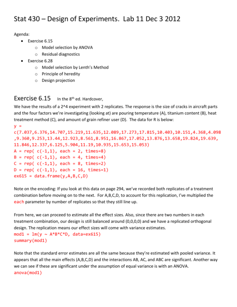
Stat 430 – Design of Experiments. Lab 11 Dec 3 2012
Agenda:
 Exercise 6.15
o Model selection by ANOVA
o Residual diagnostics
 Exercise 6.28
o Model selection by Lenth’s Method
o Principle of heredity
o Design projection
Exercise 6.15
In the 8th ed. Hardcover,
We have the results of a 2^4 experiment with 2 replicates. The response is the size of cracks in aircraft parts
and the four factors we’re investigating (looking at) are pouring temperature (A), titanium content (B), heat
treatment method (C), and amount of grain refiner user (D). The data for R is below:
y =
c(7.037,6.376,14.707,15.219,11.635,12.089,17.273,17.815,10.403,10.151,4.368,4.098
,9.360,9.253,13.44,12.923,8.561,8.951,16.867,17.052,13.876,13.658,19.824,19.639,
11.846,12.337,6.125,5.904,11.19,10.935,15.653,15.053)
A = rep( c(-1,1), each = 2, times=8)
B = rep( c(-1,1), each = 4, times=4)
C = rep( c(-1,1), each = 8, times=2)
D = rep( c(-1,1), each = 16, times=1)
ex615 = data.frame(y,A,B,C,D)
Note on the encoding: If you look at this data on page 294, we’ve recorded both replicates of a treatment
combination before moving on to the next. For A,B,C,D, to account for this replication, I’ve multiplied the
each parameter by number of replicates so that they still line up.
From here, we can proceed to estimate all the effect sizes. Also, since there are two numbers in each
treatment combination, our design is still balanced around (0,0,0,0) and we have a replicated orthogonal
design. The replication means our effect sizes will come with variance estimates.
mod1 = lm(y ~ A*B*C*D, data=ex615)
summary(mod1)
Note that the standard error estimates are all the same because they’re estimated with pooled variance. It
appears that all the main effects (A,B,C,D) and the interactions AB, AC, and ABC are significant. Another way
we can see if these are significant under the assumption of equal variance is with an ANOVA.
anova(mod1)
The linear model summary and ANOVA should give us essentially the same information when we have
replicates. It does here. Since we’re heavily dependent on the assumption of equal variance (otherwise getting
t-scores with 1 df instead of with 16 df… a huge difference), we should check if that assumption is reasonably
close to true with a residual plot.
plot(mod1$fitted, mod1$residuals)
abline(0,0)
There is a pattern; all the residual points are a mirror of another point on the negative side (the line of 0 slope,
0 intercept highlights this pattern). Is that a problem? Consider that there are two replicates per combination
and we’re currently fitting using every effect. That means the fitted values for each combination will just be
the mean of the values at that combination. There are two values in each group; one has to be above the
mean, and the other is below the mean by the same value.
Let’s try with a model using only the effects we determined to be significant earlier:
mod2 = lm(y ~ A+B+C+D + A:B + A:C + A:B:C, data=ex615)
anova(mod2)
plot(mod2$fitted, mod2$residuals)
The residuals are still in pairs, but they’re no mirrors. No other pattern has emerged. Let’s also check the
residuals against each of the main effects in one big window.
par(mfrow = c(2,2)) # sets the graphics window to show 4 plots in a 2x2 square
plot(ex615$A, mod2$residuals)
plot(ex615$B, mod2$residuals)
plot(ex615$C, mod2$residuals)
plot(ex615$D, mod2$residuals)
par(mfrow = c(1,1)) # sets it back to 1 plot at a time
The points fall into two lines because there are only two levels each of A,B,C, and D takes. The points in each
line appear to be equally spread out. This is probably enough justification to use the assumption of equal
variance.
Finally, for the smallest cracks, we’d probably recommend that the high level for C is used (its main effect and
lowest order interaction are negative), low levels for B and D (positive main effects). The level for A is a tough
call because the main effect is positive but its interaction with C is negative.
Exercise 6.28
In a replicated orthogonal design, the analysis is relatively straightforward:
1) estimate coefficients (and therefore effect sizes),
2) estimate variance of coefficient estimates,
3) compare coefficient estimates to their variance,
4) check assumption of equal variance.
When there is only one sample at each treatment combination, we have an unreplicated experiment and we
cannot estimate every coefficient and their variance at the same time. Without an estimate of the variance,
we can’t compare things against it to determine if something is significant or not.
This should be intuitive because part of a effect being significant is that we would expect to see it again if we
did the experiment over. Replicates are our way of “doing an experiment over” by doing it multiple times in
one shot.
Instead, we have to use non-parametric methods like Lenth’s Method to divine which effects are significant.
Lenth’s method splits effect sizes into large and small, and treats the small effect sizes as if they are the
variance.
We’ll need to do this in exercise 6.28 to start our analysis because it only has one replicate.
The data is:
y = c(12,18,13,16,17,15,20,15,10,25,13,24,19,21,17,23)
A = rep( c(-1,1), each = 1, times=8)
B = rep( c(-1,1), each = 2, times=4)
C = rep( c(-1,1), each = 4, times=2)
D = rep( c(-1,1), each = 8, times=1)
Runorder = c(5,9,8,13,3,7,14,1,6,11,2,15,4,16,10,12)
ex628 = data.frame(y,A,B,C,D,Runorder)
Start by getting the coefficients of the saturated model, and, since this is an orthogonal design, the effect sizes
by multiplying the coefficients by 2.
mod3 = lm(y ~ A*B*C*D, data=ex628)
summary(mod3)
effects = mod3$coef * 2
Important!!! I forgot to do this is the last time we used Lenth’s method: The intercept is just the grand mean, it
isn’t estimating any effect. So to keep it from contaminating our analysis, it should be removed from the effect
size list before continuing. The following code will toss the first element of effects (the one corresponding to
the intercept.
effects = effects[-1]
We’re assuming most of the effects are actually zero and our estimates are normally distributed around zero.
Some of these effects might not follow that pattern. These are the ones we want to keep an eye on.
qqnorm(effects)
qqline(effects)
There are some strong deviations from the normal quantile line. What are they?
xpos = qqnorm(effects)$x
ypos = qqnorm(effects,cex=0.1)$y
text(x=xpos,y=ypos,labels=names(effects))
qqline(effects)
…the main effects A, C, D, and the interactions AC and AD are all far from the normal line. We can use Lenth’s
method (described in the Nov 26 lab) to find which of these are (likely) significant.
First, get the pseudostandard error (PSE)
s0 = 1.5 * median( abs(effects))
noise = which(abs(effects) < 2.5*s0)
pse = 1.5 * median( abs(effects)[noise])
Then use that to get the margin of error (ME). We won’t bother with the simultaneous margin of error SME
because this won’t be out final word on significance.
d = length(effects) / 3
me = -qt(0.025, df=d) * pse
Last, identify effects larger than the margin of error
which( abs(effects) > me)
Lenth’s Method says that A, D, AC, and AD are significant, which agrees with our Q-Q plot assessment except
that the main effect C is missing. We may want to include C anyways because of the interaction AC. If an
interaction is significant, the main effects (or lower-order interactions) that made it also tend to be and are
assumed to be significant as well. This is called the principle of heredity. See “effect heredity” in Example 8.1,
page 326-7 for more details if you’re interested.
Heredity is automatically assumed in R when we use A*C instead of A:C
Now we can build a model using only those effects that Lenth’s Method found significant (and C). That way
we’ll have some degrees of freedom to use for estimating error.
mod4 = lm(y ~ A + D + A*C + A*D, data=ex628)
summary(mod4)
anova(mod4)
But wait, there’s more! Notice that in model 4 above, none of the significant effects involve the factor B. That
tells us that factor B has no effect on the response, not even in the interactions. That means that B can be
reasonably treated as if it weren’t a factor at all.
We can project our original 24 design onto a simpler 23 design using A,C, and D as our factors.
When we do this the response for the treatment combinations “ac” and “abc” are treated as if they were both
from “ac”, because factor B is no longer being used. We get eight such pairs from our 16 original treatment
combinations. These eight pairs are eight treatment combinations with two replicates each. We’ve
discovered some hidden replication!
In short, by disregarding the non-significant factor B, we’ve turned a 24 design with 1 replicates into a 23
design with 2 replicates. This whole process is called Design Projection. See page 260 right after example 6.2
for details.
The big advantage to design projection is interpretability. We’re looking at every main effect and interaction
that could matter among three factors, instead of looking at specific main effects and interactions. The model
below is the projected 23 design.
mod5 = lm(y ~ A*C*D, data=ex628)
summary(mod5)
anova(mod5)