STA 6167 – Exam 3 – Spring 2015 PRINT Name __________________________________________________________
Conduct all tests at  = 0.05 significance level.
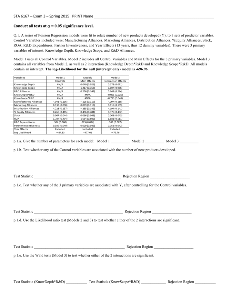
Q.1. A series of Poisson Regression models were fit to relate number of new products developed (Y), to 3 sets of predictor variables.
Control Variables included were: Manufacturing Alliances, Marketing Alliances, Distribution Alliances, %Equity Alliances, Slack,
ROA, R&D Expenditures, Partner Inventiveness, and Year Effects (13 years, thus 12 dummy variables). There were 3 primary
variables of interest: Knowledge Depth, Knowledge Scope, and R&D Alliances.
Model 1 uses all Control Variables. Model 2 includes all Control Variables and Main Effects for the 3 primary variables. Model 3
contains all variables from Model 2, as well as 2 interaction (Knowledge Depth*R&D and Knowledge Scope*R&D. All models
contain an intercept. The log-Likelihood for the null (intercept only) model is -696.96.
Variables
Knowledge Depth
Knowledge Scope
R&D Alliances
KnowDepth*R&D
KnowScope*R&D
Manufacturing Alliances
Marketing Alliances
Distribution Alliances
% Equity Alliances
Slack
ROA
R&D Expenditures
Partner Inventiveness
Year Effects
Log Likelihood
Model1
Controls
#N/A
#N/A
#N/A
#N/A
#N/A
−.041 (0.116)
0.138 (0.098)
−.223 (0.137)
0.265 (0.465)
0.067 (0.044)
1.787 (0.494)
.564 (0.080)
0.039 (0.040)
Included
−484.83
Model2
Main Effects
0.040 (0.021)
1.217 (0.358)
0.256 (0.142)
#N/A
#N/A
−.125 (0.119)
0.069 (0.113)
−.235 (0.142)
0.436 (0.484)
0.066 (0.043)
1.664 (0.506)
.525 (0.084)
0.029 (0.042)
Included
−477.01
Model3
Interaction Effects
0.178 (0.071)
3.107 (0.986)
0.643 (0.284)
-0.051 (0.025)
-0.713 (0.349)
−.097 (0.118)
0.116 (0.109)
−.194 (0.141)
0.376 (0.492)
0.063 (0.043)
1.681 (0.511)
.553 (0.087)
0.051 (0.042)
Included
−475.76
p.1.a. Give the number of parameters for each model: Model 1 __________ Model 2 __________ Model 3 __________
p.1.b. Test whether any of the Control variables are associated with the number of new products developed.
Test Statistic ______________________________________________ Rejection Region _____________________
p.1.c. Test whether any of the 3 primary variables are associated with Y, after controlling for the Control variables.
Test Statistic _______________________________________________ Rejection Region _____________________
p.1.d. Use the Likelihood ratio test (Models 2 and 3) to test whether either of the 2 interactions are significant.
Test Statistic ________________________________________________ Rejection Region _____________________
p.1.e. Use the Wald tests (Model 3) to test whether either of the 2 interactions are significant.
Test Statistic (KnowDepth*R&D) ___________ Test Statistic (KnowScope*R&D) _____________ Rejection Region ___________
Q.2. A logistic regression model was fit relating whether or not a brand was recognized 2-3 weeks after the subject had been exposed
to a comedic violent advertisement. There were two factors: Intensity of Violence (X 1=1 if High, 0 if Low) and Consequence of
Violence (X2 = 1 if Severe, 0 if Moderate). The response is Y=1 if Brand is Recognized, 0 if not. Let =Pr{Brand is Recognized}.
Consider 3 Models:
  
Model 1: log 
  0  2 X 2
 1  
  
Model 2: log 
   0  1 X 1   2 X 2
 1  
  
Model 3: log 
   0  1 X 1   2 X 2  3 X 1 X 2
 1  
The summaries for each model are given below. The table gives the estimated regression coefficients (standard errors). For the null
(intercept only) model, -2(log-Likelihood) is 25.0664.
Intercept
X1 (Intensity)
X2 (Consequence)
X1*X2
-2(log-Likelihood)
Model1
-0.20 (0.24)
#N/A
0.75 (0.34)
#N/A
20.07
Model2
-0.47 (0.29)
0.56 (0.34)
0.76 (0.34)
#N/A
17.39
Model3
-0.27 (0.33)
0.15 (0.48)
0.38 (0.46)
0.84 (0.69)
15.91
p.2.a. Based on Model 1 (and the null model), test whether there is a significant Severity of Consequence effect. H0:2=0 HA:2≠0:
Wald Test Statistic: ________________________________ Wald Rejection Region: _________________________
Likelihood Ratio Test Statistic: _________________________________ LR Rejection Region: __________________________
p.2.b. Test whether after controlling for Consequence, either Intensity or the interaction is significant: H 0: 
Test Statistic: _______________________________________
Rejection Region: _________________________
p.2.c. Based on Model 2, give the predicted probabilities of brand recognition for the 4 treatment conditions.
Intensity\Consequence
Low (X1=1)
High (X1=0)
Moderate (X2=0) Severe (X2=1)
Q.3. An Analysis of Covariance was fit, relating Trophic Level (Y) to Year (5 years, using 4 dummy variables), adjusting for Total
Length (X). The authors fit 3 models for Pacific Cod (n = 146 fish measured over the study period). The dummy coding for Year is:
Z1 = 1 if Year = 2001, 0 otherwise; Z2 = 1 if Year = 2002, 0 otherwise; Z3 = 1 if Year = 2003, 0 otherwise; Z4 = 1 if Year = 2004, 0
otherwise. Year=2000 is the “reference” year.

Model 1: E(Y) = X

Model 2: E(Y) = X + 1Z1 + 2Z2 + 3Z3 + 4Z4

Model 3: E(Y) = X + 1Z1 + 2Z2 + 3Z3 + 4Z4+ 1XZ1 + XZ2 + 3XZ3 + XZ4
SSE1 = 88.80
SSE2 = 77.85
^
Y  3.778  0.010 X  0.003Z1  0.099 Z 2  0.141Z 3  0.031Z 4
SSE3 = 75.39
p.3.a. Test H0: No interaction between year and total length (
Test Statistic: _______________________ Rejection Region: ___________________________ P-value > 0.05
< 0.05
p.3.b. Assuming no interaction, Test H0: No Year effect, controlling for total length (   
Test Statistic: _______________________ Rejection Region: ___________________________ P-value > 0.05
< 0.05
p.3.c. Based on model 2, give the adjusted means for each year (X-bar = 61.410)
Year=2000 __________ Year=2001 __________ Year=2002 __________ Year=2003 __________ Year=2004 __________
Q.4. A nonlinear regression model was fit, relating winning race speed for the Kentucky Derby winning horse (Y, in mph) to year (X,
ranging from 1896 to 2014, with n=119). For biological reasons, an S-shaped logistic function was fit (that is not limited to fall
between 0 and 1). The model fit is:
 e  2  X i  3  
E Yi    0   1   0  
 1  e 2  X i  3  


 0  0, 1  0,  2  0, 3  0
p.4.a. What occurs to E(Yi) when Xi - 3 ↓ -∞ ?
i ) E Yi    0
ii ) E Yi   1
iii ) E Yi   1   0
iv ) E Yi  
 0  1
iii ) E Yi   1   0
iv ) E Yi  
 0  1
iii ) E Yi   1   0
iv ) E Yi  
 0  1
2
p.4.b. What occurs to E(Yi) when Xi =  3?
i ) E Yi    0
ii ) E Yi   1
2
p.4.c. What occurs to E(Yi) when Xi - 3 ↑ +∞ ?
i ) E Yi    0
ii ) E Yi   1
2
The estimated regression coefficients are given below:
Coeff




Estimate Std. Error
15.36
0.2874
16.49
0.048
0.0636
0.0234
1924
9.4
p.4.d. Obtain a 95% Confidence Interval for the estimated maximum top mean speed for horses in this race.
p.4.e. Obtain a 95% Confidence Interval for 3.
p.4.f. Give the predicted time and residual for the 2014 race. The actual speed was 16.27
Q.5. Among Union (northern) soldiers during the U.S. Civil War, soldiers were classified by Rank (X 1 = 1 if Private, 0 if higher rank)
and by their duty (X2 = 1 if Infantry, 0 if not Infantry). A Poisson Regression model of the following form was fit (there was no
Interaction between rank and duty) for a sample of soldiers. Below is the model (t i is the number of soldiers exposed in that group) and
the data and regression summary.
 
log  i   0  1 X1i   2 X 2i
 ti 
i
X_1i
1
2
3
4
X_2i
1
1
0
0
Y_i
1
0
1
0
t_i
353
67
21
6
2720
1191
283
101
Coefficient Estimate StdError

-3.2952
0.2218

0.4505
0.1986

0.7964
0.1280
p.5.a. Based on a Wald test, test whether there is a Rank Effect.
H 0: _______________ HA: _________________
Test Statistic __________________________ Rejection Region ___________________________
p.5.b. Based on a Wald test, test whether there is a Duty Effect.
H 0: _______________ HA: _________________
Test Statistic __________________________ Rejection Region ___________________________
p.5.c. What are the estimated relative risks of Mortality (Private/Higher Rank) and (Infantry/non-Infantry)
Private/Higher Rank ______________________________________
Infantry/non-Infantry ________________________________
Q.6. For the Women’s National Basketball Association (WNBA) 2013 season, each game has a point spread given by oddsmakers.
Let Y = 1 if the Away team wins a game, 0 if the Away team loses. The point spread is what the Away team is supposed to get for a
bet to be fair. Thus, if the spread for the Away team is +5.5, they can lose the game by up to 5 points and still win the bet. If the
Spread for the Away Team is -5.5, they must win by more than 6 points to win the bet. Let X be the point spread for a game.
We fit a model of the form: Prob{Team Away Team Wins Game} = P Y  1   
e 0  1 X
1  e0  1 X
p.6.a. Suppose oddsmakers randomly select point spreads without taking into account team skills, injuries, or other factors. What
would that imply for 1?
1 < 0 1 = 0 1 > 0
p.6.b. Suppose oddsmakers have very good skill in selecting point spreads. What would that imply for 1? 1 < 0
1 = 0
1 > 0
p.6.c. The estimated regression coefficients, standard errors, and Wald (Z) tests are given below. Obtain fitted values when X = -10,
X = 0, and X = 10.
Coefficients:
Estimate Std. Error z value Pr(>|z|)
(Intercept) -0.155
0.162 -0.960
0.337
Away.Sprd
-0.099
0.023 -4.357 1.32e-05 ***
^
^
^
 10  __________________  0  __________________  10  __________________
p.6.d. Compute a 95% Confidence Interval for the Odds Ratio = (odds(Win|Spread=X+1)/odds(Win|Spread=X))
Lower Bound _______________________
Upper Bound _________________________
Have an Excellent Summer Break!