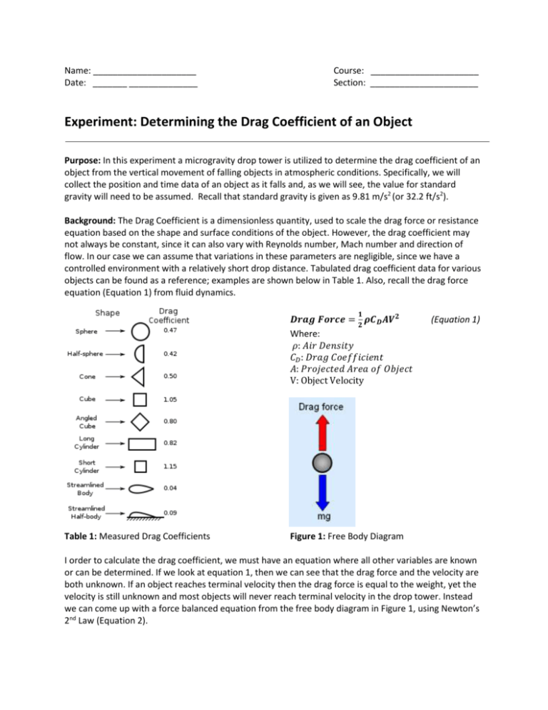
Name: _____________________
Date: _______ ______________
Course: ______________________
Section: ______________________
Experiment: Determining the Drag Coefficient of an Object
Purpose: In this experiment a microgravity drop tower is utilized to determine the drag coefficient of an
object from the vertical movement of falling objects in atmospheric conditions. Specifically, we will
collect the position and time data of an object as it falls and, as we will see, the value for standard
gravity will need to be assumed. Recall that standard gravity is given as 9.81 m/s2 (or 32.2 ft/s2).
Background: The Drag Coefficient is a dimensionless quantity, used to scale the drag force or resistance
equation based on the shape and surface conditions of the object. However, the drag coefficient may
not always be constant, since it can also vary with Reynolds number, Mach number and direction of
flow. In our case we can assume that variations in these parameters are negligible, since we have a
controlled environment with a relatively short drop distance. Tabulated drag coefficient data for various
objects can be found as a reference; examples are shown below in Table 1. Also, recall the drag force
equation (Equation 1) from fluid dynamics.
𝟏
𝑫𝒓𝒂𝒈 𝑭𝒐𝒓𝒄𝒆 = 𝝆𝑪𝑫 𝑨𝑽𝟐
𝟐
Where:
𝜌: 𝐴𝑖𝑟 𝐷𝑒𝑛𝑠𝑖𝑡𝑦
𝐶𝐷 : 𝐷𝑟𝑎𝑔 𝐶𝑜𝑒𝑓𝑓𝑖𝑐𝑖𝑒𝑛𝑡
𝐴: 𝑃𝑟𝑜𝑗𝑒𝑐𝑡𝑒𝑑 𝐴𝑟𝑒𝑎 𝑜𝑓 𝑂𝑏𝑗𝑒𝑐𝑡
V: Object Velocity
Table 1: Measured Drag Coefficients
(Equation 1)
Figure 1: Free Body Diagram
I order to calculate the drag coefficient, we must have an equation where all other variables are known
or can be determined. If we look at equation 1, then we can see that the drag force and the velocity are
both unknown. If an object reaches terminal velocity then the drag force is equal to the weight, yet the
velocity is still unknown and most objects will never reach terminal velocity in the drop tower. Instead
we can come up with a force balanced equation from the free body diagram in Figure 1, using Newton’s
2nd Law (Equation 2).
𝑵𝒆𝒘𝒕𝒐𝒏′ 𝒔 𝟐𝒏𝒅 𝑳𝒂𝒘: ∑ 𝑭 = 𝒎𝒂
Where:
𝐹: 𝐹𝑜𝑟𝑐𝑒𝑠 𝐴𝑐𝑡𝑖𝑛𝑔 𝑜𝑛 𝑂𝑏𝑗𝑒𝑐𝑡
𝑚: 𝑂𝑏𝑗𝑒𝑐𝑡 𝑀𝑎𝑠𝑠
𝑎: 𝐴𝑐𝑐𝑒𝑙𝑒𝑟𝑎𝑡𝑖𝑜𝑛 𝑑𝑢𝑒 𝑡𝑜 𝐺𝑟𝑎𝑣𝑖𝑡𝑦
(Equation 2)
The forces acting on a falling object in atmosphere are the drag force (air resistance) and the weight
(W=mg: mass*standard gravity), as shown in figure 1. Rewriting equation 1, assuming these are the only
forces acting on the object, yields the appropriate force balance. What is the equation?
Now we have an equation consisting of both the object’s instantaneous acceleration and velocity.
However, the drop tower is only capable of displaying position and time data. Therefore, we must
integrate the equation derived previously with respect to time. Equations 3-6 show that integrating
twice yields an equation in which all variables are measureable, excluding the drag coefficient.
1
𝜌𝐶𝐷 𝐴𝑉 2 − 𝑚𝑔
2
𝑎=
(𝐸𝑞𝑢𝑎𝑡𝑖𝑜𝑛 3)
𝑚
𝑑𝑉 𝑑𝑥 2
𝑎=
= 2
𝑑𝑡
𝑑 𝑡
(𝐸𝑞𝑢𝑎𝑡𝑖𝑜𝑛 4)
2𝑚𝑔
𝜌𝐶𝐷 𝐴𝑔
𝑉(𝑡) = √
∗ tanh (√
∗ 𝑡)
𝜌𝐶𝐷 𝐴
2𝑚
(𝐸𝑞𝑢𝑎𝑡𝑖𝑜𝑛 5)
𝑥(𝑡) = √
2𝑚
𝜌𝐶𝐷 𝐴𝑔
∗ ln [𝑐𝑜𝑠ℎ (√
∗ 𝑡)]
𝜌𝐶𝐷 𝐴
2𝑚
(𝐸𝑞𝑢𝑎𝑡𝑖𝑜𝑛 6)
Assuming the object starts from rest (zero initial conditions) equation 6 is derived. The object’s mass and
projected area, the air density, and the value of standard gravity will all be given. Now we can collect the
necessary position and time data from the drop tower.
Procedure: See drop tower instruction manual (also save data to file)
Results: (fill in the chart below)
Fall Height
# Object
(meter)
1
2
3
4
5
Fall Time
(sec)
Drag
Coefficient, CD
Approx.
Tabulated CD
% Difference
Conclusions:
1. Rewrite equation 6, solving for the drag coefficient.
Hint: This cannot be done algebraically, so continue to question #2 once you prove to yourself
that this is true.
2. Root finding methods from numeric methods must be used to solve equation 6 for the drag
coefficient. Use any method and program you desire, but a template is given below for the
secant method in MatLab. Simply copy and paste the code into MatLab and fill in the missing
parameters, if you so desire.
function [ Cd ] = secant_Drag(g,m,rho,A,t,x)
%Secant_Drag: Finds the drag coefficient, CD, from the non-uniform
%
equation derived from the free body diagram of a falling %
object in atmospheric conditions
% Input: m
= Mass of object
%
rho = Density of air (based on pressure)
%
A
= Projected area of object
%
t
= Fall time
%
x
= Fall height
%
Output: Cd = Drag Coefficient
clear
clc
syms Cd
f=?
x0=?
% 1st initial estimate of the root
x1=?
% 2nd initial estimate of the root
Es=0.0001;
% Desired percent error
Ea=1000; %Percent error in the root
while Ea>Es
xn=?
Ea=?
x0=x1;
x1=xn;
end
Cd=xn;
end
Hint:
3. Do the tabulated drag coefficient values compare favorably to the calculated results for any of
the objects?
4. Could the differences significantly affect the results of gravity calculations from the previous
experiments?
5. What sources of error might have affected the measurements?