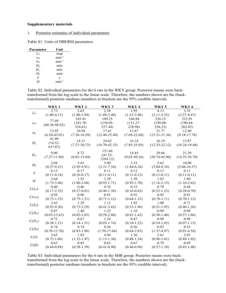
Supplementary materials
1.
Posterior estimates of individual parameters
Table S1. Units of DBERM parameters
Parameter
L0
w0
b0
HL
Hw
Hb
δ
Ω
Unit
resp
min-1
min-1
min
min
min
s
min-1
Table S2. Individual parameters for the 6 rats in the WKY group. Posterior means were backtransformed from the log scale to the linear scale. Therefore, the numbers shown are the (backtransformed) posterior medians (numbers in brackets are the 95% credible interval).
L0
w0
b0
HL
Hw
Hb
δ
Ω
C(L0)
C(w0)
C(b0)
C(HL)
C(Hw)
C(Hb)
C(δ)
C(Ω)
WKY 1
2.73
(1.80-4.11)
77.49
(60.28-98.82)
13.95
(6.54-43.01)
41.99
(14.52637.87)
WKY 2
2.63
(1.80-3.94)
243.41
(181.70324.61)
10.94
(7.36-16.59)
WKY 3
2.58
(1.89-3.48)
189.25
(158.05227.44)
17.61
(12.40-25.40)
WKY 4
1.95
(1.23-3.08)
166.84
(121.27228.94)
13.47
(7.69-22.68)
WKY 5
4.13
(3.11-5.52)
226.15
(199.00256.23)
21.77
(15.21-31.36)
WKY 6
3.35
(2.57-4.47)
222.91
(190.44262.03)
12.60
(9.18-17.78)
14.11
(7.27-30.72)
24.62
(16.70-42.32)
16.14
(7.85-35.05)
16.19
(12.25-22.12)
13.87
(10.24-19.48)
14.45
(9.03-50.16)
29.66
(20.74-45.90)
21.39
(14.35-38.70)
3.33
(1.84-6.24)
0.12
(0.11-0.12)
1.30
(0.95-1.70)
0.33
(0.16-0.62)
0.91
(0.64-1.23)
1.02
(0.53-1.96)
1.10
(0.01-1.42)
0.47
(0.10-1.22)
0.56
(0.64-2.83)
1.36
(0.88-1.24)
0.67
(0.46-0.96)
5.62
(3.84-8.18)
0.11
(0.11-0.11)
1.63
(1.16-2.15)
0.79
(0.52-1.23)
0.93
(0.78-1.11)
1.00
(0.51-1.92)
0.99
(0.56-1.40)
0.90
(0.54-1.65)
0.92
(1.37-4.97)
2.61
(0.96-1.01)
0.79
(0.57-1.18)
10.00
(5.66-16.57)
0.11
(0.11-0.11)
1.80
(1.10-2.62)
0.44
(0.28-0.70)
0.91
(0.70-1.12)
0.71
(0.40-1.26)
0.98
(0.57-1.66)
0.98
(0.07-1.15)
0.53
(0.91-4.54)
2.03
(0.89-1.02)
0.69
(0.45-1.08)
9.00
(7.27-11.80)
8.72
(6.03-15.84)
2.04
(0.37-9.21)
0.13
(0.11-0.14)
2.64
(1.75-3.46)
0.40
(0.17-2.32)
0.95
(0.75-1.25)
3.43
(0.92-9.20)
0.87
(0.03-13.63)
0.72
(0.38-1.21)
0.74
(0.59-12.70)
2.63
(0.72-1.06)
0.63
(0.44-0.89)
5.65
(2.95-9.91)
0.17
(0.16-0.17)
1.52
(1.06-2.04)
0.46
(0.27-0.81)
0.96
(0.75-1.31)
1.29
(0.73-2.29)
1.40
(0.02-2.83)
0.67
(0.14-1.51)
0.74
(0.83-3.88)
1.83
(1.32-1.47)
0.85
(0.58-1.39)
131.66
(41.532284.12)
5.00
(3.31-7.34)
0.11
(0.11-0.11)
1.28
(0.93-1.71)
0.76
(0.46-1.38)
0.91
(0.71-1.12)
1.12
(0.41-3.65)
1.25
(0.59-2.80)
1.24
(0.03-1.74)
0.56
(1.59-17.68)
4.94
(1.15-1.30)
0.63
(0.41-0.90)
Table S3. Individual parameters for the 6 rats in the SHR group. Posterior means were backtransformed from the log scale to the linear scale. Therefore, the numbers shown are the (backtransformed) posterior medians (numbers in brackets are the 95% credible interval).
SHR 1
0.47
(0.36-0.65)
351.24
(258.53480.14)
34.16
(26.74-44.23)
4017.92
(42.392.41×106)
L0
w0
b0
HL
38.50
(21.57-93.57)
Hw
Hb
δ
Ω
C(L0)
C(w0)
C(b0)
C(HL)
C(Hw)
C(Hb)
C(δ)
C(Ω)
2.
5.47
(3.93-7.47)
0.11
(0.11-0.11)
3.21
(2.51-3.97)
1.51
(1.03-2.19)
0.62
(0.35-0.97)
0.61
(0.38-0.84)
0.44
(0.00-731.64)
1.55
(0.73-3.74)
1.82
(1.13-2.80)
1.00
(0.97-1.00)
0.36
(0.26-0.50)
SHR 2
0.98
(0.82-1.22)
297.99
(256.22351.87)
27.92
(23.53-33.46)
1626.86
(81.776.49×105)
317.87
(87.037723.90)
14.42
(9.05-22.18)
0.11
(0.11-0.11)
5.25
(2.65-7.71)
1.49
(1.04-2.12)
0.75
(0.59-0.96)
0.73
(0.55-0.94)
47.93
(2.031.87×104)
1.82
(0.22-10.00)
2.49
(1.57-3.94)
1.00
(0.98-1.00)
0.40
(0.27-0.76)
SHR 3
1.74
(1.33-2.44)
125.33
(101.66154.88)
39.80
(32.19-48.62)
2001.86
(70.417.94×105)
SHR 4
2.72
(1.49-5.17)
95.74
(83.43110.95)
63.81
(47.22-83.32)
4249.27
(62.111.94×106)
SHR 5
0.29
(0.19-0.43)
240.07
(140.26382.09)
43.25
(37.36-49.92)
5400.15
(60.072.16×106)
SHR 6
0.96
(0.83-1.13)
898.68
(769.831047.51)
67.41
(57.98-78.29)
1653.46
(87.115.86×105)
45.44
(30.08-78.45)
15.21
(12.43-19.47)
18.25
(10.16-46.38)
39.42
(28.54-59.16)
8.18
(6.53-10.30)
0.11
(0.11-0.11)
2.12
(1.38-3.03)
1.56
(0.94-2.72)
1.10
(0.77-1.57)
0.79
(0.58-1.12)
39.52
(0.022.69×104)
4.35
(1.99-9.00)
2.76
(2.05-3.75)
1.00
(0.98-1.00)
0.33
(0.20-0.49)
5.82
(4.30-7.50)
0.11
(0.11-0.11)
2.03
(1.32-2.88)
1.41
(0.72-2.67)
0.70
(0.55-0.88)
0.76
(0.53-1.11)
1.62
(0.002152.52)
0.82
(0.58-1.14)
5.08
(3.40-7.50)
1.00
(0.97-1.00)
0.35
(0.23-0.54)
8.04
(7.08-9.11)
0.11
(0.11-0.11)
0.56
(0.22-1.06)
1.96
(1.19-3.34)
1.16
(0.70-2.24)
0.71
(0.56-0.88)
0.79
(0.001093.19)
2.01
(1.06-5.18)
1.84
(1.53-2.21)
1.00
(0.98-1.04)
0.43
(0.26-1.20)
7.28
(6.03-8.78)
0.11
(0.11-0.11)
4.34
(3.26-5.45)
0.91
(0.66-1.26)
0.91
(0.69-1.22)
0.78
(0.64-0.97)
70.39
(3.162.48×104)
2.65
(1.52-4.58)
1.14
(0.91-1.43)
1.00
(0.99-1.00)
0.36
(0.24-0.51)
Posterior estimates of individual parameters
It is possible that, with the low L0 of the SHR group, there were very few within-bout responses
and as a result, the parameters associated with the within-bout state cannot be estimated with high
levels of precision. Note that the converse can also be true – with a very high L0 there can be too few
bout initiations for the parameters associated with the bout-initiation state to be estimated accurately.
We tested whether the low L0 of SHR was able to detect a faster decrease in Lt (i.e., higher γ and
thus lower HL) with reasonable precision and no bias by conducting the following Monte Carlo
experiment. The posterior estimates of the DBERM parameters for individual subjects from EXT1
were retrieved. The γ of the 6 SHR rats was substituted with the γ of the 6 WKY rats. Which SHR rat
had the γ of which WKY rat was randomly assigned without replacement. Thus, this new simulated
group of 6 rats had WKY’s fast γ (and thus short HL) and SHR’s low L0 (and all other SHR rats’
parameters). Then, a Monte Carlo simulation of IRTs on EXT1 was generated for each rat using the
same method as the posterior predictive check simulation outlined in the paper. The same Bayesian
hierarchical analysis used in the paper was used to estimate this new group’s DBERM parameters.
The resultant back-transformed group median estimates were compared to SHR’s EXT1 group
medians, except for HL, which was compared to WKY’s EXT1 group median. Results in Table S4
show that (1) there was no bias in any of the group median estimates, evidenced by the 95% credible
intervals of the simulated medians covering the original medians, (2) despite the low L0, the Bayesian
analysis was able to estimate HL with reasonable precision (width of 95% CI) relative to the original
estimate for WKY (whose 95% CI is 9.35 – 55.72, see Table 1 in paper).
Table S4. Short HL can be detected despite low L0. Numbers in parenthesis are the 95% credible
interval. Original medians are from Table 1 in the paper.
Parameter
L0
w0
b0
HL
Hw
Hb
δ
Ω
Original group median
0.91 (SHR)
253.71 (SHR)
43.74 (SHR)
19.37 (WKY)
42.94 (SHR)
7.77 (SHR)
0.11 (SHR)
2.37
Median estimate of simulation
1.17 (0.30 – 4.93)
268.40 (88.36 – 812.92)
40.10 (26.18 – 62.10)
14.35 (7.57 – 27.88)
50.72 (16.27 – 830.51)
8.63 (5.34 – 14.50)
0.11 (0.11 – 0.11)
1.44 (0.10 – 8.99)
We further tested whether an even lower L0 would affect the precision with which HL could be
estimated. We took the same 6 simulated rats as above (with posterior means of SHR rats except for
HL which was from WKY rats). We lowered each rat’s L0 by multiplying them by e-1 (0.36). The
Monte Carlo IRT simulation and Bayesian hierarchical analysis was repeated. The reference group
median for L0, originally from the SHR group, was also multiplied by 0.36 to reflect the change. The
resultant “original median” for L0 was thus lowered to 0.33, i.e., one within-bout response for every
three bout initiation responses. Results in Table S5 show that (1) there was no bias in any of the
estimates of group medians, (2) estimate of HL still has reasonable precision. This shows that estimate
of HL and its precision are relatively unaffected by very low L0, suggesting that the long HL estimate
of the SHR group in the paper was not due to L0 being too low. Interestingly, a very low L0 reduced
the precision Hw estimates. This is because there were very few within-bout responses to begin with,
and because bout length declined early in the session, there was almost no within-bout response data
late in the session for Hw to be accurately estimated, and therefore the data were consistent with a
wide range of Hw values. Note however that despite this lack of precision, there was no bias in the
estimate of Hw, and that the 95% covered the original median.
Table S5. Low HL can be detected despite very low L0. Numbers in parenthesis are the 95% credible
interval. Original medians are from Table 1 in paper except that for L0.
Parameter
L0
w0
b0
HL
Hw
Hb
δ
Ω
Original group median
0.33 (Lowered)
253.71 (SHR)
43.74 (SHR)
19.37 (WKY)
42.94 (SHR)
7.77 (SHR)
0.11 (SHR)
2.37 (SHR)
Median estimate of simulation
0.31 (0.14 – 0.61)
265.36 (112.21 – 597.18)
45.97 (29.05 – 72.44)
13.75 (5.53 – 42.54)
895.49 (16.17 – 9.18×105)
7.40 (4.59 – 12.43)
0.11 (0.11 – 0.11)
2.32 (0.50 – 8.84)
3. Log survivor plots of IRTs.
Figure S1. Log survivor plots of IRTs from 4 different extinction periods from individual
WKY rats. Dots show data, while the predicted log survival probabilities as generated using
Monte Carlo simulation using samples of the posterior estimates of DBERM parameters are
shown as solid line (median) and broken lines (central 95 percentile). The number of
observed IRTs contained in each period is also shown.
Figure S2. Log survivor plots of IRTs from 4 different extinction periods from individual
SHR rats. Dots show data, while the predicted log survival probabilities as generated using
Monte Carlo simulation using samples of the posterior estimates of DBERM parameters are
shown as solid line (median) and broken lines (central 95 percentile). The number of
observed IRTs contained in each period is also shown.
4. Current data analysis compared to Cheung et al [19].
A previous paper by Cheung et al [19] references the current data set for illustrative purposes.
The results presented there are the same, except that [19] only examined EXT1, the lower
bounds for parameter estimates were set to e-15 for [19] and e-20 for the current paper. Despite
the difference in lower bounds, parameter estimate of EXT1 agreed between the two analyses
– all of the median DBERM parameters of EXT1 in this paper lie within the 95% CI of [19]
(see their Table 4), and vice versa. Both papers also found the same effect of strain on EXT1.
However, the median estimates (and their 95% CI) are not identical because (1) lower bounds
are different, and (2) the stochastic nature of MCMC means that parameter estimates will
differ slightly between analyses on the same data set even with the exact same priors and
model. The magnitude of this difference will decrease to zero as the number of MCMC
samples used tends to infinity.