Lab 4 - A Problem of Randomness
In this laboratory exercise you will study the generation and testing of pseudo-random
sequences using a computer. You will generate normally distributed random samples from
uniformly distributed samples and evaluate the normal distribution by computing the mean and
standard deviation.
Introduction - We will study a method of generating pseudorandom number sequences in which
we start with a seed value and use it to generate a random number and a new seed value for
generating the next number in the sequence. Each seed value will generate a specific random
number so that if we started with the same seed, we would generate the same sequence of
random numbers. This brings up another issue with the computer as a generator of random
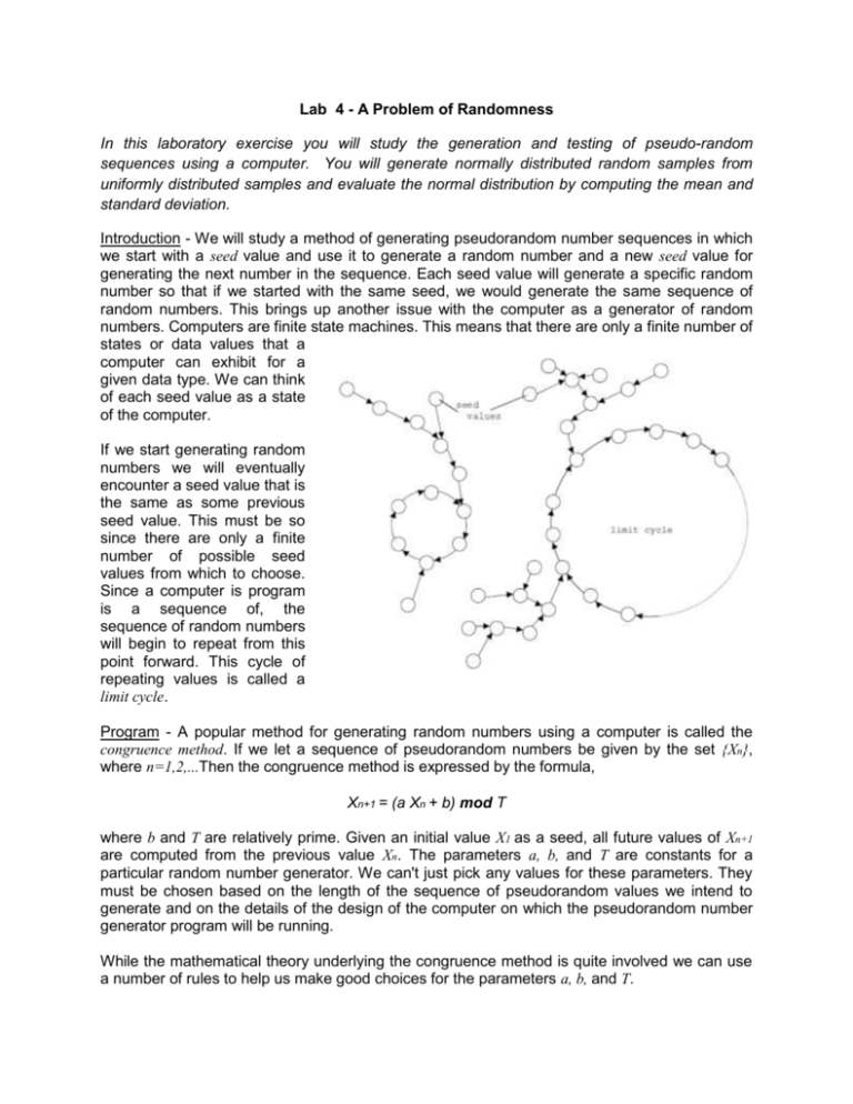
numbers. Computers are finite state machines. This means that there are only a finite number of
states or data values that a
computer can exhibit for a
given data type. We can think
of each seed value as a state
of the computer.
If we start generating random
numbers we will eventually
encounter a seed value that is
the same as some previous
seed value. This must be so
since there are only a finite
number of possible seed
values from which to choose.
Since a computer is program
is a sequence of, the
sequence of random numbers
will begin to repeat from this
point forward. This cycle of
repeating values is called a
limit cycle.
Program - A popular method for generating random numbers using a computer is called the
congruence method. If we let a sequence of pseudorandom numbers be given by the set {Xn},
where n=1,2,...Then the congruence method is expressed by the formula,
Xn+1 = (a Xn + b) mod T
where b and T are relatively prime. Given an initial value X1 as a seed, all future values of Xn+1
are computed from the previous value Xn. The parameters a, b, and T are constants for a
particular random number generator. We can't just pick any values for these parameters. They
must be chosen based on the length of the sequence of pseudorandom values we intend to
generate and on the details of the design of the computer on which the pseudorandom number
generator program will be running.
While the mathematical theory underlying the congruence method is quite involved we can use
a number of rules to help us make good choices for the parameters a, b, and T.
1. Let T be one larger than the limit of the range of values to be generated 0..(T-1).
2. Make b relatively prime to T
3. Let a = 1 (mod p) (i.e. a mod p = 1) where p is a prime factor of T or a= 1(mod 4)
if 4 is a factor of T.
Following these rules will ensure that the pseudorandom sequence of numbers generated will
cover the range of value 0..T-1 and that the sequence will pass the standard tests for
randomness.
Uniform Distribution - The congruence method generates pseudorandom sequences in an
interval (0.0..1.0) which means that each value generated will be greater than 0.0 and less than
1.0. Since any value in this range is equally likely we call the distribution uniform.
Normal Distribution - Imagine that you are throwing darts at the bull's-eye of the dartboard. The
distribution of the darts on the board will be distributed around the bull's-eye with (hopefully)
more darts closer to the center. This is an example of a normal distribution (also called a
Gaussian distribution). The bull's-eye is the mean of the distribution. If you are an expert dart
player the spread of the darts, also called the standard deviation, will be small. If you are a
beginner the spread in the darts will be larger.
While this is a two-dimensional example, we can consider the simpler case of a onedimensional or single-variable normal distribution with mean and standard deviation . The
curves shown below the dartboards represent the probability that a particular dart will land
within a specified distance from the center (or mean). We can express the probability density
as,
We can compute the probability that a dart will fall between horizontal positions x1 and x2 by
integrating the probability density function p(x) between x1 and x2. Unfortunately, this integral is
not solvable analytically but can be approximated numerically using a computer program. This
integral is also called the error function.
The mean,  and the standard deviation,  can be computed for a collection of values xi by,
where N is the number of values in the set of values being evaluated. For now we will limit
ourselves to the task of generating pseudorandom number sequences with a normal
distribution. Using the so-called direct method, we can produce normally distributed random
values from uniformly distributed random values Normal using the formula.
where R1 and R2 are two independent, uniformly distributed, random values in the
range(0.0..1.0), log( ) is the logarithm, and cos( ) is the cosine. Even though a proof of the
validity of this relationship is beyond the scope of this exercise we can implement this method in
a Java program.
Implementation - Java provides a built-in random number generator Math.random() that returns
a value in the range (0.0..1.0) each time it is called. We first need to test this method to verify
that the sequence of values generated are reasonably random. There are many tests for
randomness. In this exercise we will verify that Math.random() generates a uniformly distributed
sequence by counting the number of values in each 1/10 interval between 0.0 and 1.0.
Uniform Distribution Test Procedure
You may create your own uniform distribution generator or you may use the built-in random
number generator Math.random( ).
1. Create a list of ten integers to hold the count for each 1/10 interval.
2. Generate a sequence of uniform random number using the method being tested
3. For each random value add one to the count of the appropriate bin.
4. Compare the counts in each bin. There should be apx. 1/10 the numbers in each
It is important ant to note that the count will not be exactly the same but, in repeated trials, the
count should tend toward the same average number. You may use a series of 10 if statements
to accumulate the counts or you might use some other method. These alternative methods will
be discussed in class and in the laboratory.
Normal Distribution Test Procedure
You will build your own method for generating normally distributed random numbers using the
direct method described above. This formula produces normally distributed random numbers
with a zero mean and unit standard deviation. In order to test your normal distribution random
number generator you can compute the mean a standard deviation of a collection of value
generated using your method. The test procedure is,
1. Create an array of doubles to hold the random numbers to be generated
2. Decide on the number of values, then generate and store them in the array.
3. Compute and save the mean of these values.
4. Use the mean and the list of values to compute the standard deviation.
5. Compare the mean and standard deviation to the values expected.
Questions:
1. Did you use the built-in uniform number generator or did you create your own? ___________
2. About what percentage variation in bin count did you notice for any given trial? ___________
3. Were the bins with the lowest counts the same for each trial? _________
4. Did the uniform generator appear to produce uniformly distributed random values? ________
5. How many samples did the normally distributed generator produce each trial? ____________
6. For a zero mean and unit standard deviation how often was the mean >0.0? _____________
7. How often was the mean < 0.0? ________________
8. How often was the standard deviation > 1.0? ______________
9. How often was the standard deviation < 1.0? ______________
10. Did the normal generator appear to produce normal distributed random values? _________
Submission - Print a hardcopy of your program source code, a summary of your test method,
and the test results you obtained.