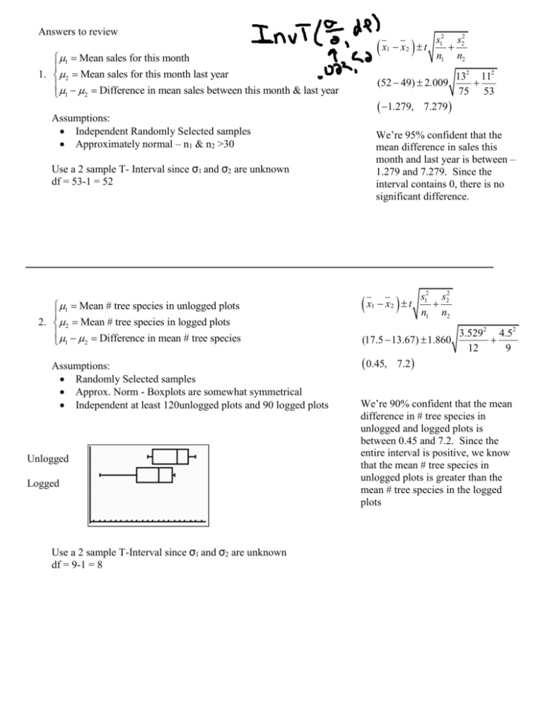
Answers to review
x
1
 1  Mean sales for this month

1.  2  Mean sales for this month last year
     Difference in mean sales between this month & last year
2
 1
 1.279,
Unlogged
Logged
Use a 2 sample T-Interval since σ1 and σ2 are unknown
df = 9-1 = 8
7.279 
132 112

75 53
We’re 95% confident that the
mean difference in sales this
month and last year is between –
1.279 and 7.279. Since the
interval contains 0, there is no
significant difference.
Use a 2 sample T- Interval since σ1 and σ2 are unknown
df = 53-1 = 52
Assumptions:
 Randomly Selected samples
 Approx. Norm - Boxplots are somewhat symmetrical
 Independent at least 120unlogged plots and 90 logged plots

(52  49)  2.009
Assumptions:
 Independent Randomly Selected samples
 Approximately normal – n1 & n2 >30
 1  Mean # tree species in unlogged plots

2.  2  Mean # tree species in logged plots
     Difference in mean # tree species
2
 1
 x2
s12 s22
t

n1 n2


x1  x 2  t
s12 s22

n1 n2
(17.5  13.67)  1.860
 0.45,
7.2 
3.5292 4.52

12
9
We’re 90% confident that the mean
difference in # tree species in
unlogged and logged plots is
between 0.45 and 7.2. Since the
entire interval is positive, we know
that the mean # tree species in
unlogged plots is greater than the
mean # tree species in the logged
plots
 s 
xd  t  d 
 n
3.
 3.33 
3.11  3.355 

 9 
 6.839, 0.6171
d  Before - After
Assumptions:
 Dependent (Paired) random samples
 Approximately normal
Since boxplot of differences is somewhat symetrical
Before - After
We’re 99% confident that the
mean difference in the # hours
spent studying before and after
the seminar is between -6.839hr
and 0.6171hr. Since the interval
contains 0, there is no significant
difference between them.
Use a Matched Pairs T-Test
df = 9 – 1 = 8
 p1  Proportion of males opposed to death penalty

p q
p q
4.  p2  Proportion of females opposed to death penalty
p1  p 2  z 1  2
 p  p  Difference in prop. of males & females opposed to death penalty
n1
n2
2
 1
.4(.6) .56(.44)
(.4  .56)  1.96

Assumptions:
200
100
 Randomly Selected Samples
 0.2786,  0.0414 
 Approximately normal


Independent – at least 2000 females and 1000 males
𝑛1 𝑝̂1 = 80 > 10
𝑛1 𝑞̂1 = 120 > 10
𝑛2 𝑝̂2 =56>10
𝑛2 𝑞̂2 = 44 > 10
Use a 2-Proportion Z-Interval

We’re 95% confident that the
difference in Proportion of
females and males opposed to the
death penalty is between 0.2786
and 0.0414. Since the entire
interval is negative, we know that
the proportion of females opposed
to the death penalty is greater
than the proportion of males who
are opposed to the death penalty.
 p1  Proportion of registered voters in CA who voted

5.  p2  Proportion of registered voters in CO who voted
 p  p  Difference in proportion of regitered voters in CA & CO who voted
2
 1
 H o : p1  p2

 H A : p1  p2
z
Assumptions:
 Independent Randomly Selected samples
 Approximately normal since

z
𝑛1 𝑝̂1 = 141 > 10
𝑛1 𝑞̂1 = 147 > 10
𝑛2 𝑝̂2=123>10
𝑛2 𝑞̂2 = 93 > 10
 p  p  p  p  
1
2
1
2
1 1 
pc qc   
 n1 n2 
.49  .57   0
1 
 1
.523(.477) 


 288 216 
p  value  0.038
pc 
Use the 2-Proportion Z-Test
 1.77
141  123 264

 0.523
288  216 504
Reject the Ho since p-value<α.
There’s sufficient evidence to support the
claim that the proportion of voter turnout in
Colorado is higher than that in California.
6. d  typewriter-computer
 H o : d  0

 H A : d  0
Assumptions:
 Matched Pairs Dependent random samples
 Boxplot symmetrical – population
Is approximately normal
x d  d

sd
n
6.2  0
t
 3.398
5.77
10
p  value  0.004
df  9
t
Reject the Ho since p-value <α.
There’s sufficient evidence to support the
claim that the secretaries can type more
words per minute using computers rather
than typewriters.
Use a matched pairs T-Test
df = 9-1 = 8
7. p  proportion of murders committed by women
 H o : p  0.10

 H A : p  0.10
z
z
Assumptions:
 Simple random sample
 Approximately normal since
np  67(.10)  7  5
nq  67(.90)  60  5
p p

pq
n
.15  .1
 1.34
.1(.9)
67
p  value  0.18
Fail to reject the Ho since p-value > α.
Use a 1-proportion Z-Test
There’s insufficient evidence to support
the claim that the proportion of murders
committed by women is not 10%.
 1  Mean amount administrators pay for hosp. insurance

8.  2  Mean amount nurses pay for hosp. insurance
     Difference in mean amount paid by administrators & nurses
2
 1
 H o : 1  2

 H A : 1  2
t
Assumptions:
 Independent random samples
 Approx Norm since boxplots are somewhat symm.
t
Admin
Nurses
Use the 2-Sample T-Test since σ1 and σ2 are unknown
x
1

 x 2   1   2 
s12 s22

n1 n2
 55  60.92   0
5.062 4.22

12
12
3.11
p  value  0.003
df  11


Reject the Ho since p-value<α.
There’s sufficient evidence to support the
claim administrators pay less for
hospitalization insurance than nurses.
 1  Mean score for math majors

9.  2  Mean score for computer science majors
     Difference in score for math & computer majors
2
 1
 H o : 1  2

 H A : 1  2
Assumptions:
 Independent random samples
 Approximately normal since
n1 & n2 >30
Use the 2-Sample T- Interval since σ1 and σ2 are unknown
t
t
x
1

 x 2   1   2 
s12 s22

n1 n2
 83.6  79.2   0
4.32 3.22

36
49
p  value  0
 5.18
Reject the Ho since p-value<α.
There’s sufficient evidence to support the
claim that there is a difference in scores
between math & computer majors on the
test.
  Mean score on the exam
10. .
 H o :   75

 H A :   75
Assumptions:
 Simple random samples
 Population normal – distribution
Is not normal since n < 30
scores
Use the 1-Sample T-Test since σ1 is unknown
x

s
n
70.85  75
t
 2.83
6.56
t
20
p  value  0.0108
=0.004
df  19
Reject the Ho since p-value < α.
There’s sufficient evidence to support the
claim that the mean test score is different
from 75.