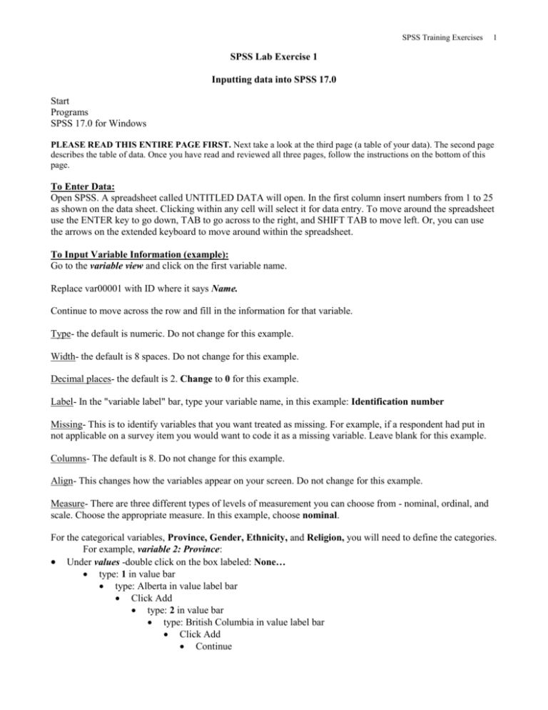
SPSS Training Exercises
1
SPSS Lab Exercise 1
Inputting data into SPSS 17.0
Start
Programs
SPSS 17.0 for Windows
PLEASE READ THIS ENTIRE PAGE FIRST. Next take a look at the third page (a table of your data). The second page
describes the table of data. Once you have read and reviewed all three pages, follow the instructions on the bottom of this
page.
To Enter Data:
Open SPSS. A spreadsheet called UNTITLED DATA will open. In the first column insert numbers from 1 to 25
as shown on the data sheet. Clicking within any cell will select it for data entry. To move around the spreadsheet
use the ENTER key to go down, TAB to go across to the right, and SHIFT TAB to move left. Or, you can use
the arrows on the extended keyboard to move around within the spreadsheet.
To Input Variable Information (example):
Go to the variable view and click on the first variable name.
Replace var00001 with ID where it says Name.
Continue to move across the row and fill in the information for that variable.
Type- the default is numeric. Do not change for this example.
Width- the default is 8 spaces. Do not change for this example.
Decimal places- the default is 2. Change to 0 for this example.
Label- In the "variable label" bar, type your variable name, in this example: Identification number
Missing- This is to identify variables that you want treated as missing. For example, if a respondent had put in
not applicable on a survey item you would want to code it as a missing variable. Leave blank for this example.
Columns- The default is 8. Do not change for this example.
Align- This changes how the variables appear on your screen. Do not change for this example.
Measure- There are three different types of levels of measurement you can choose from - nominal, ordinal, and
scale. Choose the appropriate measure. In this example, choose nominal.
For the categorical variables, Province, Gender, Ethnicity, and Religion, you will need to define the categories.
For example, variable 2: Province:
 Under values -double click on the box labeled: None…
 type: 1 in value bar
 type: Alberta in value label bar
 Click Add
 type: 2 in value bar
 type: British Columbia in value label bar
 Click Add
 Continue
SPSS Training Exercises
 OK
Enter all the data and name all the variables in this manner, according to the description provided. Repeat this
sequence for all the variables.
Data Description
Var1
Var2
Var3
Var4
Var5
Var6
Var7
Respondent's identification number (ID)
Province the respondents lives in (PROVINCE)
1
Alberta
2
British Columbia
Respondent's gender (GENDER)
1
male
2
female
Respondent's ethnicity (ETHNICITY)
1
Caucasian
2
Black
Respondent's age (AGE)
Respondent's religious affiliation (RELIGION)
1
Protestant
2
Catholic
3
Jewish
4
None
5
Other
Respondent' s mother‘s education - years of schooling (MAEDUC)
Name your data set and save it the data (either to disk or to your student file)
Note: Use this data to complete Exercise 1 Part B.
2
SPSS Training Exercises
DATA SET
1
2
3
4
5
6
7
8
9
10
11
12
13
14
15
16
17
18
19
20
21
22
23
24
25
id
province
gender
ethnicity
age
religion
maeduc
1
2
3
4
5
6
7
8
9
10
11
12
13
14
15
16
17
18
19
20
21
22
23
24
25
1
1
1
1
1
1
1
1
1
1
1
1
2
2
2
2
2
2
2
2
2
2
2
2
2
1
2
2
2
1
1
2
1
2
1
2
2
2
1
1
1
2
1
1
2
1
2
1
2
2
1
1
2
1
1
1
2
2
2
2
1
2
2
1
2
1
1
1
1
2
2
2
1
2
1
32
37
72
86
30
32
29
29
53
68
19
43
38
45
24
53
20
27
54
25
20
38
20
34
67
1
2
2
3
1
2
1
1
1
1
2
2
4
2
4
2
2
2
2
1
2
2
2
2
1
16
13
20
12
5
10
18
4
6
9
2
14
12
17
1
3
7
11
8
15
1
7
5
10
19
3
SPSS Training Exercises
4
SPSS Lab Exercise 2
Running Frequencies and Descriptives in SPSS 17.0
There are 2 ways to retrieve the data file you saved in exercise 1:
a)
Enter SPSS. An untitled data sheet will appear. Click on File. Click on Open. Click on arrow under Drives: Click
on a: (or relevant drive) Under file name, click on the file (.sav). OK.
b)
Click on My Computer icon. Click on or relevant drive. Click on data file (.sav). SPSS will be initiated and the
data will appear.
Open previous data file from Exercise 1.
Task 1
To run frequencies for each variable, with the data editor open in the data view, go to:











Analyze
Descriptive Statistics
Frequencies
Click on the selected variable in the left box and transfer it to the Variable(s) box by clicking the arrow. Note: You can
transfer more than one variable to the Variable(s) box and run frequencies for all variables at the same time.
In the same window click on Statistics
Select minimum, maximum, and range (they may already be selected as default)
Continue
In the same window click on Charts…
Bar chart (You can also try a histogram with or without the normal curve, and a pie chart. However, SPSS will only
allow you to select on 1 chart at a time!)
Continue
OK
If you want you may name your output and save it. The computer will give the output an ‘.spv’ extension if you are using
SPSS 17 or an ‘.spo’ extension if you are using another version of SPSS. This indicates that your frequencies are saved as
an output file.
Run frequencies for the following categorical (i.e., discrete) variables: Gender, Ethnicity, Religion, and Province.
Answer the following questions:
What percentage of the sample is female?
____________
What percentage of the sample is Black?
____________
What percentage of the sample is Catholic?
____________
What percentage of the sample is from Alberta?
____________
Task 2
To run Descriptives for each variable go to:
 Analyze
 Descriptive Statistics
 Descriptives
 Click on the selected variable in the left box and transfer it to the Variable(s) box by clicking the arrow. You can
transfer more than one variable to the Variable(s) box and run descriptives for all variables at the same time.
 In the same window click on Options
SPSS Training Exercises



Select mean, standard deviation, minimum, maximum and range (some may already be selected as default)
Continue
OK
If you want to you may name your output and save it.
Run Descriptives for the continuous variables: Age, and Mother’s Education (maeduc).
Fill in the following table.
Variable
Mean
Standard
Deviation
Lowest Value
Highest Value
Range
Age
Mother’s Education
(in years)
Task 3
Now we want to review the process of cutting and pasting from your SPSS output into a Microsoft Word document.
SPSS output should currently be open on the computer screen in front of you. Let's copy the Descriptives table you just had
SPSS produce and paste it into a "hypothetical" Microsoft Word document.
In order to copy and paste, you must:
1.
Go back to the bottom left corner of your computer screen to the command Start. Click on Start. Click on Programs.
Find Microsoft Word. Click on Microsoft Word. The Microsoft Word program should open up onto your computer
screen.
2.
Sometimes the Microsoft Word program will now ask you what you want to do. If the program asks, you want to
create a new document.
3.
Minimize your Microsoft Word program by clicking on the first of the three small boxes at the top right hand side of
your screen. The box you want is gray, square, and contains only a small line through the box.
4.
Now your SPSS output screen should be open in front of you.
5.
Using your mouse, click once on the Descriptives table. The Descriptives table should now be surrounded by a box.
6.
Using your mouse, move your pointer to the top of the SPSS output screen to the command Edit. Click on Edit.
7.
Click on Copy Objects.
8.
Now minimize your SPSS output screen by clicking on the first of the three small boxes at the top right hand side of
your screen. The box you want is gray, square, and contains only a small line through the box.
9.
Your Microsoft Word program should now be in front of you.
10. Click anywhere on the screen. There should now be a blinking cursor. Move the cursor down several lines (in case you
want to add a title or a sentence about the SPSS descriptives table) by clicking on Enter several times.
11. Using your mouse, click on the Edit command at the top of your screen. Click on Paste.
12. Your SPSS Descriptives table should now appear in your Microsoft Word document. The Microsoft Word table
should be identical to the SPSS table.
5
SPSS Training Exercises
SPSS Lab Exercise 3
Frequencies
Data manipulation: Recoding and Selecting Cases.
Central Tendency Measures
Histograms
Task 1
Open your data file from Exercise 1.
Imagine that you need to classify your respondents into five categories in terms of their ages. To do so you will need to
create a new categorical variable.
Recode the continuous variable Respondent's Age (age) into a new categorical variable (agegroup).
The values for the new variable will be as follows:
New Values (agegroup)
Old values (age):
1 – late adolescent
2 – young adult
3 – middle adult
4 – late adult
18-20
21-40
41-60
61-90
Note: The width of these intervals are not equal. In a true study, we would want the interval widths to be consistent!
In the menu bar go to Transform

Recode
 Into different variable…
 Transfer “age” into Output variable box
 Type the name of a new variable - agegroup
 Click on Change
 Click on Old and New Values
 In Old values select Range and type the first range of the old values: 18-20
 In New value type 1
 Click on Add
 Repeat these steps for all old and new values
 Continue
 OK
You should have a new variable (agrgroup) with the values 1 to 4.
Now define the new variable and its value levels. (You do this under variable view)
Now obtain the frequencies for agegroup:
What age group category has the least number of participants/people? _________
What age group category has the most number of participants/people? _________
What % of the sample is late adult?
_________
What % of the sample is young adult?
_________
What % of the sample is middle adult?
_________
6
SPSS Training Exercises
7
Task 2
Run the frequencies for the following variables: maeduc and age.
Now find the standard deviation, variance, minimum and maximum values for these variables.
To do so, in the main menu bar go to:

Analyze
 Descriptive Statistics
 Frequencies
 Click on the selected variables in the left box and transfer them to the Variable(s) box by clicking the right
arrow.
 In the same window click on Statistics…
 Select appropriate statistics
 Continue
 Charts…
 Histogram
 Select Display normal curve
 Continue
 OK
Variable
Age
Mean
Median
Mode
Maximum
Shape
Maeeduc
Task 3
Run frequencies for the variables age and years separately for males and females.
To do this we need to select the cases according to respondent's gender.
To run the frequencies for each gender we will first select males, run the frequencies for males, and then select females and
run the frequencies for females.
To select males:

Go to Data
 Select cases
 If condition is satisfied
 If…gender =1 (Select Gender, click arrow, then select function =1)
 Continue (Please note: Unselected cases should be FILTERED as deleting the cases will delete
them forever!)
 OK
You have now selected only the males. Until you re-select everyone, reset the select feature, or select only females, all the
statistics you do from this point forward will be based only on males!
Next we need to run the frequencies:

Analyze
 Descriptive Statistics
 Frequencies
 Statistics
 Move maeduc and age variables into Variable(s) box.
SPSS Training Exercises

Click on the boxes of standard deviation, variance, skewness, minimum, maximum, mean, mode,
and median.
 Continue
 OK
Your SPSS output will present your frequencies for males only. Note your sample size is smaller then it was during task 2.
We have excluded the females from this analysis!
Next, you will have to repeat these steps for analyzing the data for females.
Before selecting females you will need to reset the data. In order to do so go to
 Data
 Select Cases
 Reset
Now select only females using the following procedure and then re-run the frequency analysis.

Go to Data
 Select cases
 If condition is satisfied
 If…gender =2 (Select Gender, click arrow, then select function =2)
 Continue (Please note: Unselected cases should be FILTERED as deleting the cases will delete
them forever!)
 OK
Use your output to answer the following questions:
Variable
Age/ M
Mean
Median
Mode
St. deviation
Variance
Shape
Maeduc/ F
Now produce the histogram with normal curve for these variables.
Remember to select cases appropriately for each variable.
In the main menu bar go to:

8
Graphs
 Histogram
 Transfer appropriate variable to Variable bar
 Select Display normal curve
 OK
Another way to obtain the frequencies for males and females separately would have been to go to:
 Data
o Split File
 Compare Groups
 Click on “Organize output by groups”
o Move the gender variable from the left box into the middle box under
“Groups Based On”
 Click OK.
In order to unsplit the file, go back to Split File and select “Analyze all cases, do not create groups”.
SPSS Training Exercises
9
ADDITIONAL SPSS TECHNIQUES
Simple Correlation
Task 1: Correlation between Two Variables
Use the 1991 U.S. General Social Survey.dat data set (ITS website) to find the strength of the relationship
between fathers’ education level (highest year of school completed, father: paeduc) and mother’s education level
(highest year of school completed, mother: maeduc).
In the main menu bar go to:
 Analyze
 Correlate
 Bivariate (meaning 2 variables)…
 Transfer the appropriate set of variables to the Variable box
 The default options selected are Pearson Correlation Coefficient, 2 tailed significance test,
flag significant correlations
 OK
paeduc
paeduc
r=1.00
maeduc
maeduc
Is the correlation significant?
r=1.00
Yes / No
If yes, at what significance level?
How many people are in the data set?
What proportion of variance in maeduc is explained by paeduc? ____________
Note about interpreting significant correlations: With larger samples, small correlations may be deemed
significant because of the power. A better way of interpreting correlations is to consider the proportion of
variance (r2). For example, a correlation of 0.2 may be significant, but accounts for only 4 percent of the
variance.
Scattterplot: The scatterplot enables you to see whether a correlation will accurately summarize the relationship
between 2 variables. Correlations are appropriate only for linear relationships. The r will be an underestimation
if the relationship is curvilinear. It is important to examine scatterplots when studying relationships between
variables.
To produce a scatterplot for the pair of variables, in the main menu bar go to:
 Graphs
 Chart Builder - OK
 Select “Scatter” from the gallery
 Select “Simple” or the first graph presented – running your mouse over each example graph will tell
you what they are.
 Select the variables from the list on the upper left and drag and drop the variable on the selected
axis
 Transfer maeduc to the Y-axis and paeduc to the X-axis
 OK (The graph will then be entered into your viewer folder)
SPSS Training Exercises 10
SPSS produces simple scatterplots this way. To obtain a line of best fit (more on this next lab)
 Double click on your graph
 Chart Editor window will open
 From the menu bar in the Chart Editor window select ELEMENTS - Fit Line at Total
 OK
 Close the Chart Editor window
Describe the relationship between the maeduc and paeduc.
Task 2: Correlations for a Subset of the Sample
Determine the relationship between education (educ) and mothers education (maeduc) for male students.
Reduce your output. To select a subsample of students you need to select cases. In the main menu bar:

Data
 Select Cases
 If condition is satisfied
 If
 Move Sex into empty box on the right and create statement specifying the gender of interest
(i.e., sex = 1 will specify males)
 Continue
 OK
Now run the correlation (analyze, correlate, biverate) and produce the scatterplot.
Male respondents
Education
Mother’s Education
Education
Mother’s Education
What proportion of variance in Education is explained by Mother’s Education for male students? ____________
What do you conclude?
Before running further analyses, you need to unselect the cases (Data, Select Cases, All Cases, OK).
SPSS Training Exercises 11
Independent Samples and Dependent Samples t-tests
Task 1: Confidence Intervals
Using the GSS93 subset.sav data set (located within the SPSS program or on the ITS website), you will make
interval estimates (confidence intervals) of the parameters for the adult population of the United States.
To get the confidence intervals you will need to go to:
 Analyze
 Descriptive Statistics
 Explore
 Transfer your variable to the Dependent List.
 Select Statistics: Descriptives and specify the appropriate Confidence Interval for the Mean.
 Continue, OK
1. What is the average number of years of education (mean highest level of education) of the females adult
population?
Number of Cases
Mean
95% Confidence Interval
Lower Bound
Upper Bound
Years of Education (educ)
Task 2: Testing a Hypothesis About Two Related Means
Use the Anxiety2.sav data set (ITS website).
1. Create a new variable that is the difference between trial 1and trial 4 anxiety (variables trial1 and trial4)
Go to:
 Transform
 Compute
 Type "diff" in target variable box
 Click on " trial1" and transfer it into the numeric expression box.
 Click on the subtract sign or type in "-"
 Click on " trial4" and transfer it into the numeric expression box,
 OK
Now make a Histogram of the variable "diff" (go to Graphs, Chart Builder, Select Histogram, and put diff on X
axis, OK) and examine the distribution.
1. Does the distribution appear to be normal?
____________
2. Conduct a t-test for dependent samples
 Analyze
 Compare Means
 Paired Samples T-test
 Highlight both trial1 and trial4 variables and transfer them into the Paired variables box.
 Under Options specify the confidence intervals as 95%
 Continue
 OK
3. Now answer the following questions:
a) What is the correlation between trial1 and trial4?
_______________
b) Using the 0.05 level of significance, do you reject or retain the null hypothesis? ___________
SPSS Training Exercises 12
Task 3: Testing Hypothesis About Two Independent Means
Problem: A researcher is interested in the effect of an approach to teaching graduate statistics on statistics
anxiety. The statistics course offered by the Educational Psychology department is a lecture based course and a
computer based course with no lectures. The content of both courses is exactly the same. There are twelve
students in each class. At the end of the course students were asked to fill out the Statistics Anxiety
Questionnaire. The results are presented below:
EDPY 500
Lecture Based Approach
EDPY 500
Computer Based Approach
10
23
11
17
7
4
18
11
11
14
10
19
27
24
15
19
17
21
26
17
20
29
27
22
Please enter this data into SPSS. (HINT: To do this, you will have to enter two rows of data: one for the class
(the first 12 rows will have an indicator 1 to indicate lecture and the second 12 rows will have an indicator 2 to
indicate computer) and one column for the respective anxiety scores).
Test the null hypothesis that the difference between the mean anxiety score of the students taking the lecture
based course and the mean anxiety score of the students taking the computer based course is zero.
1. Enter the data into the SPSS file and define the variables.
2. Produce the histograms and examine the distribution of the anxiety scores for both groups.
To do this go to:
 Data
 Split File
 Click on "Organize Output by Groups"
 Click on Groups Based On:
 Enter Class
 Sort File By Grouping Variable
 OK
3. Do the scores in both populations appear to be normally distributed?
4. Go Back and UNSPLIT the file. Remove "class" from Groups Based On, Click on Analyze All Cases
and then select OK.
5. Conduct a t-test for two independent samples:
 Analyze
 Compare Means
SPSS Training Exercises 13
 Independent Samples t test
 Transfer your dependent variable (anxiety) to Test Variable(s) and the independent variable
(teaching approach) to the Grouping Variable bar.
 Define the groups...
 Type the numerical values for the two groups
 Continue
 Under options select the 95% confidence interval
 Continue
 OK
6. Examine your output and answer the following questions:
a) What are the mean anxiety scores for the two groups? _____________ _____________
b) Is the assumption of homogeneity of variance met? For Levene's test for equality of variances, if
the test is nonsignificant, do not reject the hypothesis that the two population variances are equal. _________
c) What is the mean difference for the two samples?
______________
d) What is the value of the t test?
______________
e) How many degrees of freedom are there?
______________
f) What is the obtained p value?
______________
g) Using the 0.05 level of significance, do you reject or retain the null hypothesis?
______________