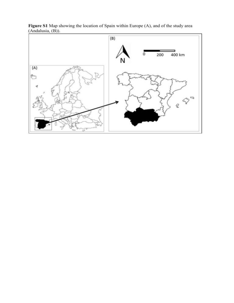
Figure S1 Map showing the location of Spain within Europe (A), and of the study area
(Andalusia, (B)).
Appendix S1 Analytical methods _ Analysis of tree survival
To analyze tree survival as a function of several environmental and biotic variables we
used adult census data for the two times, N1 and N2 in a binomial likelihood where trees
survived between censuses with probability Ѳ. Then for stand i:
N2i ~Binomial(N1i, Ѳi)
And process model:
logit(Ѳi) = αregion(i) + βXi + bi
where α is the intercept (estimated for each region, wet and dry), β represents the vector of
fixed effect coefficients associated with each of the exploratory variables included, Xi is
the matrix of explanatory variables (the final model included: winter precipitation, winter
temperature, slope, topographic radiation index, sand content, sand*winter precipitation
and heterospecific basal area, Table 1), and bi is a spatially explicit random effect.
Appendix S2 Analytical methods _ Analysis of the seedling group
In the analysis of the seedling group, we defined the likelihood using a zero inflated
Poisson distribution (Zuur et al. 2009) with mean parameter µ, due to the excess zerocounts in the data. We tried other types of models, i.e. zero inflated negative binomial, and
approaches to the ordinal data, through inclusion of a latent variable for each count (Table
S5). For the final model, the probability of a zero count was given by . The likelihood in
stand i with count yi was:
Pr(yi = 0)
𝑃𝑜𝑖𝑠𝑠𝑜𝑛(𝜔𝑖 + (1 − 𝜔𝑖 ) × 𝑒 −𝜇𝑖 )
𝑦
𝜇 𝑖
Pr(Yi=yi | yi > 0) 𝑃𝑜𝑖𝑠𝑠𝑜𝑛((1 − 𝜔𝑖 ) × 𝑒 −𝜇𝑖 × ( 𝑦𝑖 ! ))
𝑖
And process model:
ln⁡(𝜇𝑖 ) ⁡ = ⁡ 𝛾𝑟𝑒𝑔𝑖𝑜𝑛(𝑖) + 𝜑 × Χi + ⁡ ϵi + ⁡ 𝑏i
with an intercept γ for each region, fixed effect coefficients φ and a matrix of explanatory
variables, Xi that for the final model included: winter precipitation, winter temperature,
their interaction, slope and heterospecific basal area (Table 2). We also included individual
error term per stand, εi, and spatial random effects, bi.
References
Zuur, A.F., Ieno, E.N., Walker, N.J., Saveliev, A.A. & Smith, G.M. (2009) Zero-truncated
and zero-inflated models for count data (ed. by Zuur, A.F., Ieno, E.N., Walker, N.J.,
Saveliev, A.A., Smith, G.M.). Mixed effects models and extensions in ecology with
R, 261-293.. Springer, New York, New York
Appendix S3 Analytical methods _ Analysis of the sapling group
For the analysis of the sapling group we evaluated the abundance of saplings in those
stands where they were present (71 stands in total). We used a Poisson likelihood (with
parameter µ) to model the abundance of saplings recorded in the second census (SFNI3):
Pr(Yi = yi)
𝑦
𝜇 𝑖
𝑃𝑜𝑖𝑠𝑠𝑜𝑛(𝑒 −𝜇𝑖 × ( 𝑦𝑖 ! ))
𝑖
And process model similar to the model used for seedlings:
ln⁡(𝜇𝑖 ) ⁡ = ⁡ 𝛾𝑟𝑒𝑔𝑖𝑜𝑛(𝑖) + 𝜑 × Χi + ϵi⁡ + ⁡ 𝑏i
In this case the explanatory variables included in Xi for the best model were annual
temperature and precipitation in spring, but none of them were significant (Table 2, Table
S7).
Appendix S4 Analytical methods _ Parameter estimation
We followed a Bayesian approach to estimate the parameters of the adult tree survival and
recruitment models, α, β, γ, φ, ω, є and b. Bayesian modeling allowed us to track the
different sources of uncertainty inherent in the analysis, i.e., the data, the process and the
parameters (McCarthy, 2007). Parameters were estimated from non-informative prior
distributions, α, β, γ and φ ~Normal(0,1000), єi ~Normal (0, 2) with 1/2
~Gamma(0.01,0.01) and ωi~Beta(1,1). The spatial random effects bi were estimated using
Bayesian Gaussian kriging models, where the spatial random effects were estimated
separately for each region as:
bi|bj, j≠i~Normal(exp(-(ρdij)κ), b2)
where dij is the distance between two stands, ρ is the rate of decay estimated from
ρ~Gamma(1,1), the smoothing parameter, , was set up to 1, and 1/b2~Gamma(0.1,0.1).
Posterior densities of the parameters were obtained by Gibbs sampling (Geman & Geman,
1984) using OpenBUGS 3.1.2. (Thomass et al. 2006). Models were run until convergence
of the parameters was reached (~150,000 iterations) and parameters and their confidence
intervals were estimated after discarding pre-converge “burn-in” iterations (~10000). Plots
of predicted versus observed values were also used to evaluate the fit of the model
(unbiased model having a slope of unity). R2 of observed vs predicted values was used as a
measure of goodness-of-fit. Fixed effects coefficients,  and φ parameters, whose 95%
credible intervals did not include zero, were considered statistically significant.
References
Geman, S. & Geman, D. (1984) Stochastic relaxation, Gibbs distributions, and the
Bayesian restoration of images. Ieee Transactions on Pattern Analysis and
Machine Intelligence, 6, 721-741.
McCarthy M. A. (2007) Bayesian Methods for Ecology, Cambridge University Press,
Cambridge.
Thomas, A., O'Hara, R., Ligges, U. & Sturts, S. (2006) Making BUGS Open. In: R News,
6, 12-17.
Table S1 Number of stands and number of Q. suber trees (total and dead between SFNI2
and SFNI3) considered for the analysis of tree survival. Number of stands where seedlings
and saplings were present considered in the analysis of recruitment.
Analysis of tree survival
Total
Stands in SNFI2
Q. suber trees
Mean trees/stand
Tree Mortality
Number of stands
(Percentage total stands)
Trees
(Percentage total trees)
Maximum (tree/stand)
Mean (tree/stand in stands were
mortality was recorded)
Analysis of recruitment
Seedling
Stands (with present individuals)
Sapling
Stands (with present individuals)
Andalusia
Wet region
Dry region
755
4964
6.6
408
3541
8.7
347
1423
4.1
170
22.5
347
7.0
28
114
27.9
271
7.7
28
56
16.1
76
5.3
6
2.0
2.4
1.4
396/736
254/405
142/331
71/736
35/405
36/331
Table S2 Mean (± sd) and minimum and maximum values of the exploratory variables for
each region.
Variables
Climatic
Topographic
Edaphic*
Biotic
Annual temperature (ºC)
Spring temperature (ºC)
Summer temperature (ºC)
Fall temperature (ºC)
Winter temperature (ºC)
Annual precipitation (mm)
Spring precipitation (mm)
Summer precipitation (mm)
Fall precipitation (mm)
Winter precipitation (mm)
Slope %
Sand content %
Silt content %
Clay content %
Soil bulk density (g/cc)
Organic matter %
Soil water content (g/100g)
Available water capacity
(g/100g)
pH
Conspecific basal area3
(m2/ha)
Heterospecific basal area3
(m2/ha)
Wet region
mean±sd
16.8±1.1
14.8±1.2
23.4±1.0
18.1±1.1
10.9±1.3
1031.8±172.5
237.4±42.4
30.1±9.7
280.3±46.8
484.0±82.5
3.3±2.2
36.3±9.6
23.7±4.3
39.4±8.6
1.5±0.1
1.2±0.1
28.4±5.7
18.3±6.2
min
12.8
10.5
20.5
13.2
6.8
472.0
116.0
8.0
121.0
214.0
0.1
31.7
5.6
19.4
1.05
0.6
12.1
3.0
max
18.7
16.9
25.5
19.9
13.3
1756.0
390.0
57.0
506.0
812.0
11.3
70.1
33.8
56.7
1.7
1.4
36.3
21.4
Dry region
mean±sd
16.0±1.0
14.0±1.0
24.2±0.9
17.0±1.0
8.8±1.1
767.3±96.6
196.6±23.1
38.3±7.7
216.0±29.07
315.9±47.4
2.0±1.4
44.2±7.5
27.3±6.1
27.2±4.1
1.5±0.2
1.2±0.2
20.9±3.3
9.7±5.1
min
13.1
10.7
21.8
13.8
5.4
532.0
131.0
20.0
133.0
204.0
0.2
30.2
15.6
19.6
1.1
0.8
12.1
5.9
max
18.6
16.7
26.6
20.0
11.7
1092.0
257
62.0
314.0
468.0
5.3
63.5
34.8
35.8
1.7
1.4
24.7
31.6
6.7±1.0
11.5±6.8
6.1
0.4
7.0
42.1
6.4±0.3
5.5±4.9
6.1
0.4
7.1
25.8
3.8±6.3
0.0
38.0
4.7±6.6
0.0
54.2
* For soil bulk density, soil water content and available water capacity the spatial
resolution was 1:400.000. The other soil variables were estimated by the SEISnet system.
The estimates come from three levels of information: regional level, landscape levels and
field soil profiles. Average values of the soil properties of interest were estimated by using
a model based on three main information sources: (1) a Geological Mining map and (2) a
FAO soil-classes map, both at 1:400.000 scale; and (3) a wide array of detailed soil data
stored in a soil profile database of the study area (SDBm Plus, de la Rosa et al 2002).
Using pedotransfer functions (de la Rosa et al 2001) and interpolation techniques for
spatial data, average values of several soil properties of interest, for a given geo-edaphic
unit and location, were estimated (Monge et al. 2008). For a more detailed description see:
De la Rosa, D., Mayol, F., Moreno, F., Cabrera, F., Diaz-Pereira, E. & Antoine, J. (2002)
A multilingual soil profile database (SDBm Plus) as an essential part of land
resources information systems. Environmental Modelling & Software, 17, 721-730
Monge, G., Rodríguez, J.A., Anaya-Romero, M. & de la Rosa, D. (2008) Generación de
Mapas Lito-Edafológicos de Andalucía. Mapping Interactivo. Revista Internacional
de Ciencias de la Tierra, 124, 38-45.
Table S3 Factor loadings of varimax-rotated factors for the soil variables. The most
representative variables for each axis are shown in bold.
Variables
pH
Clay content
Silt content
Sand content
Organic matter
Soil water content
Soil bulk density
Available water capacity
Importance of components
Standard deviation
Proportion of variance
Cumulative proportion
Factor 1
0.48
0.92
-0.06
-0.93
0.30
0.92
0.60
0.92
Factor 2
-0.03
-0.07
0.32
-0.23
-0.14
-0.18
0.94
-0.16
Factor 3
-0.01
0.20
0.11
-0.05
0.94
0.17
-0.21
0.17
3.82
0.42
0.42
1.49
0.17
0.59
1.09
0.12
0.71
Table S4 Selected models to evaluate the probability of mature tree survival. Predictive
loss (D) and description of the best models in each group of variables (smallest value of
D). We included only the interactions that were significant. To account for spatial
autocorrelation we added a spatially random effect bi. Temperature and precipitation in the
models including topographic, soil and biotic variables correspond to temperature in spring
and precipitation in winter. αi are the intercepts for each region, βi are the parameters of the
covariates Xi.
Model description
Hierarchical
A model with the form P(Y| y)= αjs
+ βjs x Xj where αjs and βjs are the
parameters for each X1 to Xj
covariates in each s region, allowed
us to combine data from the two
regions to estimate the overall
response of cork oak to the climatic
variables while allowing for
variation in this response among the
two regions. Parameter estimation
for one region was informed by data
from the other region through the
hyperparameters aj and bj. αjs and
βjs were estimated from prior
distributions αjs~Normal(a,σa2) and
βjs~Normal(b,σb2) respectively.
Prior parameters for this
distributions were estimated from
un-informative distributions:
a~Normal(0,1000),
σa~Uniform(0,1000),
b~Normal(0,1000),
σb~Uniform(0,1000).
Simple Bayes
Climate
Climate+Topography
Climate+Soils
Climate+Biotic variables
Process model
D
logit(pi)=
α1,S+α2,S*Winter Precipitationi+α3,S*Spring Temperaturei
Observations: high values of the standard deviation of the
hypermarameters leaded us to discard the hierarchical model and work
with the two regions independently.
1402
logit(pi)=
α[regionS]+α2* Precipitationi+α3* Temperaturei
Annual temperature
1733
Winter temperature
1878
Spring temperature
1560
Summer temperature
1771
Fall temperature
2185
Spring temperature-annual precipitation
1560
Spring temperature-winter precipitation (selected)
1511
Spring temperature-spring precipitation
2087
Spring temperature-summer precipitation
1827
Spring temperature-fall precipitation
1964
logit(pi)=
α[regionS]+α2*Winter Precipitationi+α3*Spring
Temperaturei+α4*Slopei+α5*Topographic radiation indexi
logit(pi)=
α[regionS]+α2* Winter Precipitationi+α3*Spring Temperaturei+α4*Sand
contenti+α5*Soil bulk densityi+α6*Organic matteri
logit(pi)=
α[regionS]+α2*Winter Precipitationi+α3*Spring
Temperaturei+α4*Slopei+α5*Topographic radiation
indexi+α6*Sandi+α7*Sandi*Winter Precipitationi+α8*Heterospecific
basal areai
1387
1461
1496
Climate + Topographic + Soils
+ Biotic variables
Model accounting for spatial
autocorrelation
Climate + Topographic + Soils
+ Biotic variables+spatially
random effect
logit(pi)=
α[regionS]+α2*Winter Precipitationi+α3*Spring
Temperaturei+α4*Slopei+α5*Topographic radiation
indexi+α6*Sandi+α7*Sandi* Winter Precipitationi+α8*Heterospecific
basal areai
logit(pi)=
α[regionS]+α2*Winter Precipitationi+α3*Spring
Temperaturei+α4*Slopei+α5*Topographic radiation
indexi+α6*Sandi+α7*Sandi*Winter Precipitationi+α8*Heterospecific
basal areai+bi
1269
493
Table S5 Selected models to evaluate the number of Q. suber seedlings less than 1.30 m
tall. We included only the interactions that were significant. Temperature and precipitation
in the models including topographic, soil and biotic variables correspond to temperature in
winter and precipitation in winter. Mean μi of the positive count data is calculated as a
function of the covariates. γi are the intercepts for each region, φi are the parameters of the
covariates Xi. ωi was estimated with a prior distribution Beta(1,1). ki is a parameter from
the negative binomial distribution and it represents the number of failures until a certain
number of successes. D: predictive loss calculated for each model. To account for spatial
autocorrelation we added to the best models a spatially random effect bi. To account for
the overdispersion of the non-zero data we tried two different approximations: in a first
approach, we added a stand level random effect є into the linear predictor for the Poisson
intensity, µ. As a second approach, we specified a negative binomial (ZINB) distribution
that is overdispersed relative to the Poisson (Kéry 2010). Zero-inflated Poisson
distributions (ZIP) resulted in a better fit to the data compared with ZINB and accordingly
we used the ZIP model. We also considered the number of counts, yi as a latent variable,
where the true value of counts was estimated from a normal distribution with mean yi and a
variance constrained to reflect the maximum and minimum values of that ordinal level
(e.g., the low ranged from 1 to 4, we used a mean of 2 and a variance of (4-1)2/12, variance
of the uniform distribution). We tried several model structures and combination of
explanatory variables, and once the best model was selected we accounted for spatial autocorrelation by adding a spatially explicit random effect, defined above.
References
Kéry, M. (2010) Introduction to WinBUGS for Ecologists: A Bayesian Approach to
Regression, ANOVA and Related Analyses. Academic Press. Burlington, MA.
Model description
Process model
Selection of the likelihood distribution
Zero-inflated negative
Pr(yi = 0)
ωi+(1-ωi )*(ki/(μi+ki))ki
binomial
(explanatory variables
Pr(Yi=yi | yi > 0)
annual precipitation and
(1-ωi)*(Γ(yi+ki)/(Γ(ki)*Γ(yi+1))*(ki/(μi+ki))ki*(1-ki/(μi+ki))yi
temperature)
μi = exp(α0+α1*X1i+…..+αn*Xni+εi)
Zero-inflated Poisson
Pr(yi = 0)
ωi+(1-ωi )*exp(-μi)
number of
Pr(Yi=yi | yi > 0)
(1-ωi)*exp(-μi)*(μiylatenti/ylatenti!)
seedlings/saplings as a
latent variable
μi = exp( γ0+φ1*X1i+…..+φn*Xni+εi)
(explanatory variables
annual precipitation and
temperature)
Zero-inflated Poisson
number of
Pr(yi = 0)
ωi+(1-ωi )*exp(-μi)
seedlings/saplings as a fix Pr(Yi=yi | yi > 0)
(1-ωi)*e-μi*(μiyi/yi!)
variable
(explanatory variables
μi = exp( γ0+φ1*X1i+…..+φn*Xni+εi)
annual precipitation and
temperature)
Alternative groups of models with a Zero Inflated Poisson likelihood
Hierarchical
A model with the form
P(Y| y)= α1s + βjs x Xj
where αjs and βjs are the
parameters for each X2 to
Xj covariates in each s
region, allowed us to
combine data from the
two regions to estimate
the overall response of
cork oak to the climatic
variables while allowing
for variation in this
response among the two
regions. Parameter
estimation for one region
Pr(yi = 0)
ωi+(1-ωi )*exp(-μi)
was informed by data
Pr(Yi=yi | yi > 0)
(1-ωi)*e-μi*(μiyi/yi!)
from the other region
through the
μi = exp( γ1,S+γ2,S*Winter Precipitationi+φ1,S*Winter
hyperparameters aj and
Temperaturei+εi)
bj. αjs and βjs were
estimated from prior
distributions
αjs~Normal(a,σa2) and
βjs~Normal(b,σb2)
respectively. Prior
parameters for these
distributions were
estimated from uninformative distributions:
a~Normal(0,1000),
σa~Uniform(0,1000),
b~Normal(0,1000),
σb~Uniform(0,1000).
Simple Bayes
Annual temperature
D
215100
30270
15070
14950
15070
Climate+topography
Climate + edaphic
variables
Climate+ biotic
variables
Climate +
Topography +
Biotic variables
Model accounting
for spatial
autocorrelation
Climate +
Topographic +
Biotic
variables+spatially
random effect
Winter temperature
15030
Spring temperature
15210
Summer temperature
15080
Fall temperature
15040
Spring temperature-annual precipitation
15030
Winter temperature-winter precipitation (selected)
14980
Winter temperature-spring precipitation
15040
Winter temperature-summer precipitation
15050
Winter temperature-fall precipitation
15000
μi = exp(γ [regionS]+φ1* Winter Precipitationi+φ2*Winter
Temperaturei+φ3* Winter Precipitationi* Winter
Temperaturei+εi)
μi = exp(γ[regionS]+ φ1* Winter Precipitationi+ φ2* Winter
Temperaturei+ φ3* Winter Precipitationi* Winter
Temperaturei+ φ4*Slopei+φ 5*Top radiation indexi+εi)
μi = exp(γ[regionS]+φ1* Winter Precipitationi+φ2* Winter
Temperaturei+φ3* Winter Precipitationi* Winter
Temperaturei+φ4*Sand contenti+φ5*Soil bulk
densityi+φ6*Organic matteri+εi)
μi = exp(γ[regionS]+φ1* Winter Precipitationi+φ2* Winter
Temperaturei+φ3* Winter Precipitationi* Winter
Temperaturei+φ4*Conspecific basal areai+φ5*Heterospecific
basal areai+εi)
μi = exp(γ[regionS]+φ1* Winter Precipitationi+φ2* Winter
Temperaturei+φ3* Winter Precipitationi* Winter
Temperaturei+φ4*Slopei+φ5*Heterospecific basal areai+εi)
μi = exp(γ[regionS]+φ1* Winter Precipitationi+φ2* Winter
Temperaturei+φ3* Winter Precipitationi* Winter
Temperaturei+φ4*Slopei+φ5*Heterospecific basal areai+εi +bi)
14980
14960
15130
14950
14890
14680
Table S6 Classification of small seedlings (height < 0.30 m), large seedlings (height
between 0.30 m and 1.30 m), small saplings (height > 1.30 m and dbh < 2.5 cm) and large
saplings (height >1.30 m and 2.5<dbh<7.5 cm) in SFNI2 and SFNI3. The semiquantitative scale corresponds to low: 1-4 seedlings or saplings, medium: 5-15 seedlings or
saplings, or high: >15 seedlings or saplings. To make a unique category of saplings we add
the exact number of saplings in category 4 of the SIFN3 and the average count for each of
the ordinal categories for category 3 in the SIFN3 (low = 2, medium = 10, and high = 20).
The corresponding recruitment stage group column shows the two different groups
(seedlings and saplings) considered in the analysis.
corresponding
recruitment
Height
dbh
quantification
SIFN2
SIFN3
stage group
for the
analysis
< 0.30 m
-
semi-quantitative scale
category 1
category 1
seedlings
0.30-1.30 m
-
semi-quantitative scale
category 1
category 2
seedlings
>1.30 m
<2.5 cm
semi-quantitative scale
category 1
category 3
saplings
category 2
category 4
saplings
>1.30 m
2.5-7.5 cm exact number of saplings
Table S7 Predictive loss (D) for the models run in the analysis of saplings (>1.30 m high).
Alternative models
Climate
D
Annual temperature
849.5
Winter temperature
857.4
Spring temperature
855.8
Summer temperature
850.9
Fall temperature
850.8
Annual temperature-annual precipitation
849.6
Annual temperature-winter precipitation
851.3
Annual temperature-spring precipitation
847.9
Annual temperature-summer precipitation
853.9
Annual temperature-fall precipitation
851.4
Topography
853.2
Soil
850.5
Biotic
852.8
Previous recruitment census
857.1
Soil, biotic
854.5
Soil, biotic + spatially explicit random effect
850.1