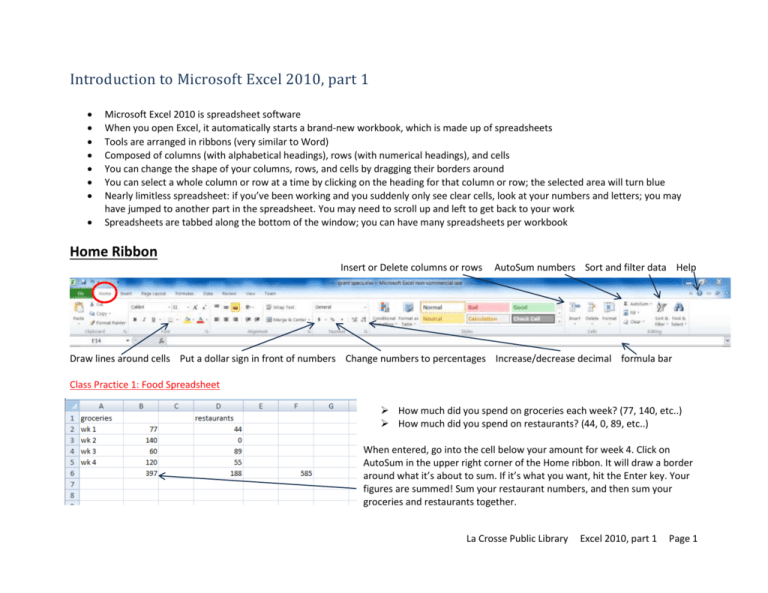
Introduction to Microsoft Excel 2010, part 1








Microsoft Excel 2010 is spreadsheet software
When you open Excel, it automatically starts a brand-new workbook, which is made up of spreadsheets
Tools are arranged in ribbons (very similar to Word)
Composed of columns (with alphabetical headings), rows (with numerical headings), and cells
You can change the shape of your columns, rows, and cells by dragging their borders around
You can select a whole column or row at a time by clicking on the heading for that column or row; the selected area will turn blue
Nearly limitless spreadsheet: if you’ve been working and you suddenly only see clear cells, look at your numbers and letters; you may
have jumped to another part in the spreadsheet. You may need to scroll up and left to get back to your work
Spreadsheets are tabbed along the bottom of the window; you can have many spreadsheets per workbook
Home Ribbon
Insert or Delete columns or rows
AutoSum numbers Sort and filter data Help
Draw lines around cells Put a dollar sign in front of numbers Change numbers to percentages Increase/decrease decimal formula bar
Class Practice 1: Food Spreadsheet
 How much did you spend on groceries each week? (77, 140, etc..)
 How much did you spend on restaurants? (44, 0, 89, etc..)
When entered, go into the cell below your amount for week 4. Click on
AutoSum in the upper right corner of the Home ribbon. It will draw a border
around what it’s about to sum. If it’s what you want, hit the Enter key. Your
figures are summed! Sum your restaurant numbers, and then sum your
groceries and restaurants together.
La Crosse Public Library
Excel 2010, part 1
Page 1
You can adjust the AutoSum border by clicking on one of the four corners of the box and dragging it up or down (or side to
side). Once you’ve outlined what you wish to sum, hit the Enter key.
You can also adjust the AutoSum border by clicking your mouse on a different cell and dragging down and/or across to make
the selection.
The formula bar shows the contents of a particular cell. If you use AutoSum or another
formula, you can see the math here. This example shows that Excel is going to sum the contents of cells B3 through B6.
You can rename your spreadsheet down at the bottom of the window. Double-click on the word
“Sheet1” and type in a new name.
Class Practice 2: Donor Spreadsheet
Click on “Sheet2” to start a new spreadsheet in the same workbook.

Who donated how much?
Enter in names and amounts. One way to sort your data is by first clicking on the
square in the corner between 1 and A to select all of your cells; then click on the
Sort & Filter button in the upper right corner of the Home ribbon. Excel will keep
your rows intact (Joe will still have donated 3700, Bob 45.5, etc.).
Did your column headings (name, donation) get sorted into the mix? Undo your sort
(either using the undo arrow in the upper left corner of the window or by hitting
ctrl+z). Select all of your cells again, then go to Sort & Filter and choose Custom Sort.
Make sure the box next to “My data has headers” is checked! Click OK.
La Crosse Public Library
Excel 2010, part 1
Page 2
What percentage of the total was Joe’s donation? You can enter your own
formula by choosing a blank cell and using the formula =sum(one cell
number/another cell number). In this example, you’d type in =sum(B2/B5) to
get .81.
Class Practice 3: Loan Due Date Spreadsheet

When is the loan due?
You can add together dates and numbers to figure out a future (or past) date. In this example, your
formula in cell B4 would look like =sum(B2:B3).
Note: sometimes you’ll see a green triangle in the upper left corner of a cell. This is Excel’s way of
alerting you that the formula omits adjacent cells (for instance, our autosum didn’t include cell B1).
File Ribbon
Much like in Word, you go to File to save, open, print, or start a new workbook. Note: in Excel 2007, File is replaced by a circular icon:
Under New, there are many premade templates to
explore. A blank workbook is selected by default.
You can see a small preview in the right pane.
Once you’ve selected the type of workbook you’d
like to open, click on Create.
La Crosse Public Library
Excel 2010, part 1
Page 3
Print preview pane
Saving
Choose Save if you’re
comfortable saving over
the previous version of
your workbook. Use Save
As if you’re not sure you
want to permanently keep
your changes.
Save early, save often!
Printing
Click here to print
You can change your print
settings here. Type in
specific page numbers to
print if you don’t want
them all to print; you can
also change orientation,
page size, margins, and
scaling (printing at actual
size, fitting all columns on a
page, fitting all rows on a
page, etc).
Learn more printing options in Excel 2010, part 2.
Note: in Excel 2007, you’ll have to choose Print Preview to see
what your spreadsheet looks like before printing.
Number of pages in spreadsheet (click the triangles to preview
other pages)
Last updated 10/14/13
La Crosse Public Library
Excel 2010, part 1
Page 4