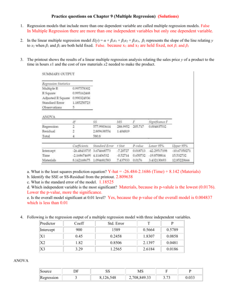
Practice questions on Chapter 9 (Multiple Regression) (Solutions)
1. Regression models that include more than one dependent variable are called multiple regression models. False
In Multiple Regression there are more than one independent variables but only one dependent variable.
2. In the linear multiple regression model E(y) = α + β1x1 + β2x2 + β3x3, β2 represents the slope of the line relating y
to x2 when β1 and β3 are both held fixed. False. because x1 and x3 are held fixed, not β1 and β3
3. The printout shows the results of a linear multiple regression analysis relating the sales price y of a product to the
time in hours x1 and the cost of raw materials x2 needed to make the product.
a. What is the least squares prediction equation? Y-hat = -26.484-2.1686 (Time) + 8.142 (Materials)
b. Identify the SSE or SS-Residual from the printout. 2.809638
c. What is the standard error of the model. 1.18525
d. Which independent variable is the most significant? Materials, because its p-valule is the lowest (0.0176).
Lower the p-value, more the significance.
e. Is the overall model significant at 0.01 level? Yes, because the p-value of the overall model is 0.004837
which is less than 0.01
4. Following is the regression output of a multiple regression model with three independent variables.
Predictor
Coeff
Std. Error
T
P
Intercept
900
1589
0.5664
0.5789
X1
0.45
0.2458
1.8307
0.0858
X2
1.82
0.8506
2.1397
0.0481
X3
3.29
1.2565
2.6184
0.0186
ANOVA
Source
Regression
DF
SS
MS
F
P
3
8,126,548
2,708,849.33
3.73
0.033
Residual
20
14,523,685
Total
23
22,650,233
726,184.25
a. What is the least square regression line? Y-hat = 900 + 0.45.X1 + 1.82.X2 + 3.29.X3
b. What is the SSE? 14,523,685
c. If X2 and X3 are held constant and if X1 increases by 5 units, what will be the estimated average change
in y? y will increase by an estimated average value of 5 * 0.45 = 2.25
d. Which independent variable is the most significant? X3 because its p-value is the lowest.
e. Is X1 significant at 0.05 level? No (because its p-value is higher than 0.05)
f. Is the overall model significant at 0.05 level?
Yes (because the overall p-value of 0.033 is < 0.05)
g. What is the R-square value? SSR/SSyy = 8126548/22650233 = 0.3588
h. Test the hypothesis (at alpha of 0.05) that beta1 is not zero
H0 : beta1 = 0
Ha : beta1 ≠ 0
p-value = 0.0858
Fail to Reject the Null
Conclusion: Not sufficient evidence at significance level of 0.05 that beta1 is not zero.
i.
Test the hypothesis (at alpha of 0.05) that beta2 is not zero
H0 : beta2 = 0
Ha : beta2 ≠ 0
p-value = 0.0481
Reject the Null
Conclusion: There is sufficient evidence at significance level of 0.05 that beta2 is not zero.
5. Retail price data for n = 60 hard disk drives were recently reported in a computer magazine. Three variables were
recorded for each hard disk drive:
y = Retail PRICE (measured in dollars)
x1 = Microprocessor SPEED (measured in megahertz)
(Values in sample range from 10 to 40)
x2 = CHIP size (measured in computer processing units)
(Values in sample range from 286 to 486)
A linear regression model was fit to the data. Part of the printout follows:
VARIABLE
INTERCEPT
SPEED
CHIP
DF
1
1
1
PARAMETER
ESTIMATE
STANDARD
ERROR
T
PROB > |T|
-373.526392
104.838940
3.571850
1258.1243396
22.36298195
3.89422935
-0.297
4.688
0.917
0.7676
0.0001
0.3629
a. Identify and interpret the estimate for the SPEED β-coefficient, 𝑏1
A) 𝑏1 = 105; For every 1-megahertz increase in SPEED, we estimate PRICE (y) to increase $105, holding CHIP fixed.
B) 𝑏1 = 105; For every $1 increase in PRICE, we estimate SPEED to increase 105 megahertz, holding CHIP fixed.
C) 𝑏1= 3.57; For every 1-megahertz increase in SPEED, we estimate PRICE to increase $3.57, holding CHIP fixed.
D) 𝑏1 = 3.57; For every $1 increase in PRICE, we estimate SPPED to increase by about 4 megahertz, holding CHIP fixed.
b. Identify and interpret the estimate of β2.
Estimate of β2 is b2 = 3.57; The interpretation is: for every one unit increase in CHIP size, the
Price (y) is estimated to increase by an average of $3.57, holding SPEED fixed
6.
As part of a study at a large university, data were collected on n = 224 freshmen computer science (CS) majors in
a particular year. The researchers were interested in modeling y, a student’s grade point average (GPA) after three
semesters, as a function of the following independent variables (recorded at the time the students enrolled in the
university):
x1 = average high school grade in mathematics (HSM)
x2 = average high school grade in science (HSS)
x3 = average high school grade in English (HSE)
x4 = SAT mathematics score (SATM)
x5 = SAT verbal score (SATV)
A linear regression model was fit to data. A 95% confidence interval for β1 is (.06, .22). Interpret this result.
A)
B)
C)
D)
We are 95% confident that a CS freshman’s GPA increases by an amount between .06 and .22 for every 1point increase in average HS math grade, holding x2 - x5 constant.
95% of the GPAs fall within .06 to .22 of their true values.
We are 95% confident that a CS freshman’s HS math grade increases by an amount between .06 and .22 for
every 1-point increase in GPA, holding x2 - x5 constant.
We are 95% confident that the mean GPA of all CS freshmen after three semesters falls between .06 and .22.
7. A linear regression model was fit to data with the following results:
_____________________________________________________________________
SOURCE
DF
SS
MS
F VALUE
PROB > F
MODEL
5
28.64
5.73
11.69
.0001
ERROR
218
106.82
0.49
TOTAL
223
135.46
ROOT MSE
DEP MEAN
0.700
4.635
R-SQUARE 0.211
ADJ R-SQ 0.193
Interpret the value under the column heading PROB > F.
A) There is sufficient evidence (at α = .01) to conclude that the linear model is statistically useful for predicting
GPA.
B) There is insufficient evidence (at α = .01) to conclude that the linear model is statistically useful for predicting
GPA.
C) Over 99% of the variation in GPAs can be explained by the model.
D) Fail to reject H0 (at α = .01) where H0 says that all the betas are zero.