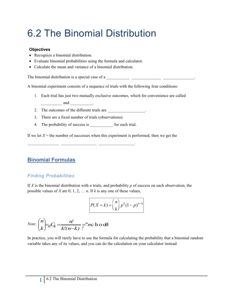
6.2 The Binomial Distribution
Objectives
 Recognize a binomial distribution.
 Evaluate binomial probabilities using the formula and calculator.
 Calculate the mean and variance of a binomial distribution.
The binomial distribution is a special case of a ___________ ______________ _______________.
A binomial experiment consists of a sequence of trials with the following four conditions:
1. Each trial has just two mutually exclusive outcomes, which for convenience are called
__________ and ___________.
2. The outcomes of the different trials are __________________.
3. There are a fixed number of trials (observations).
4. The probability of success is ___________ for each trial.
If we let X = the number of successes when this experiment is performed, then we get the
_______________ _________________ _________________.
Binomial Formulas
Finding Probabilities
If X is the binomial distribution with n trials, and probability p of success on each observation, the
possible values of X are 0, 1, 2, … n. If k is any one of these values,
æ nö
P( X = k) = ç ÷ p k (1- p) n- k
è kø
n
Note:  nCk 
k
 
n!
"nc h o ok"
se
k!( nk ) !
In practice, you will rarely have to use the formula for calculating the probability that a binomial random
variable takes any of its values, and you can do the calculation on your calculator instead.
1
6.2 The Binomial Distribution
Usually the sampling is carried out without replacement which means the trials are not independent. In
this case the number of successes observed is not a binomial distribution but a different type of
distribution called a hypergeometric distribution. Fortunately when the sample size n is much smaller
than the population size, probabilities calculated using the binomial distribution and the hypergeometric
distribution are very close in value. They are so close, that statisticians often ignore the difference and use
the binomial probabilities instead. The following guidelines are recommended for deciding whether the
binomial distribution is appropriate when sampling without replacement:
If at most 5% of the population is sampled without replacement, then the binomial distribution gives a
good approximation to the probability distribution of x.
Example 1: The number, X, of switches that fail inspection has approximately a binomial distribution
with n = 10 and p = 0.1. Find the probability that no more than one switch fails.
Example 2: About 8.8% of people ages 14-24 are “dropouts”, persons who are not in regular school and
who have not completed the 12th grade. Suppose you pick five people at random from this age group.
(a) What is the probability that none of the five are dropouts?
(b) What is the probability that at least one is a dropout?
Shape, Center and Spread
E( X )   x  n p
x  n p(1  p )
Example 3: Dolores is a 65% free throw shooter and each shot is independent. If X is the count of free
throws made by Dolores, and she makes 10 throws, what is the average and standard deviation of the
number of throws she makes?
2
6.2 The Binomial Distribution
How do the shape, center, and spread of a binomial distribution change as p increases for fixed
values of n?
The following applet illustrates how the shape, center and spread change for different values of p and n:
http://www.bilkent.edu.tr/~ktarik/econ222/applets/BinomialDist2.html
Shape:
 For small values of p the binomial distributions are highly ____________ toward the larger
values of x.

As p increases to 0.5, the distributions get more ________________, with perfect
_____________ achieved at p = 0.5.

As p increases from 0.5 to 1, the distributions get increasingly skewed toward the __________
values of x.

As n ___________, the skewness decreases for values of p different from 0.5 and the
distributions tend to look more and more _______________.
Center:

Because the mean is located at np, it ____________ with both n and p increasing.
Spread:

Similarly, the standard deviation _____________ as n increases.

For a fixed n, the standard deviation is largest around __________ and gets smaller as p gets
closer to _____ or _____.
Example 4: The median annual household income for US households is about $44,400.
(a) Among 5 randomly selected US households, find the probability that 4 or more have incomes
exceeding $44,4000.
(b) Consider a random sample of 16 US households.
i. What is the expected number of households with annual incomes under $44,400?
ii. What is the standard deviation of the number of households with annual incomes under
$44,400?
iii. What is the probability of getting at least 10 out of the 16 households with annual
incomes under $44,400?
3
6.2 The Binomial Distribution