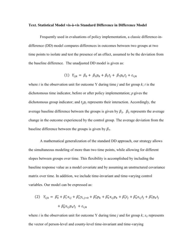
Text. Statistical Model vis-à-vis Standard Difference in Difference Model
Frequently used in evaluations of policy implementation, a classic difference-indifference (DD) model compares differences in outcomes between two groups at two
time points to isolate and test the presence of an effect, assumed to be the deviation from
the baseline difference. The unadjusted DD model is given as:
(1) 𝑌𝑖𝑗𝑘 = 𝛽0 + 𝛽3 𝑝𝑘 + 𝛽5 𝑡𝑗 + 𝛽7 𝑝𝑘 𝑡𝑗 + 𝜀𝑖𝑗𝑘
where i is the observation unit for outcome Y during time j and for group k; t is the
dichotomous time indicator, before or after policy implementation; p gives the
dichotomous group indicator; and 𝑡𝑗 𝑝𝑖 represents their interaction. Accordingly, the
average baseline difference between the groups is given by 𝛽3. 𝛽5 represents the average
change in the outcome experienced by the control group. The average deviation from the
baseline difference between the groups is given by 𝛽7.
A mathematical generalization of the standard DD approach, our strategy allows
the simultaneous modeling of more than two time points, while allowing for different
slopes between groups over time. This flexibility is accomplished by including the
baseline response value as a model covariate and by assuming an unstructured covariance
matrix over time. In addition, we include time-invariant and time-varying control
variables. Our model can be expressed as:
(2) 𝑌𝑖𝑗𝑘 = 𝛽0∗ + 𝛽1∗ 𝑥𝑖𝑗 + 𝛽2∗ 𝑦𝑖,𝑗=0 + 𝛽3∗ 𝑝𝑘 + 𝛽4∗ 𝑥𝑖𝑗 𝑝𝑘 + 𝛽5∗ 𝑡𝑗 + 𝛽6∗ 𝑥𝑖𝑗 𝑡𝑗 + 𝛽7∗ 𝑝𝑘 𝑡𝑗
+ 𝛽8∗ 𝑥𝑖𝑗 𝑝𝑘 𝑡𝑗 + 𝜀𝑖𝑗𝑘
where i is the observation unit for outcome Y during time j and for group k; xij represents
the vector of person-level and county-level time-invariant and time-varying
characteristics which we added as control variables; yi,j=0 is an individual’s compliance in
the baseline year; p is the dichotomous group indicator; and t is a categorical variable
representing time, which is allowed to have more than two levels. The DD model is a
specific case of this more generalized model.
Our approach borrows strength over time, thus increasing overall statistical
power. Under the standard DD approach, this analysis would require four paired time
comparisons; our analytic strategy allows us tocompare all four post-implementation time
points simultaneously; subsequently, we are not bound by the parallel trend assumption.
The model that we use further generalizes the DD model by allowing the baseline
difference to be any value, which is restricted to 1.0 in DD (also by the parallel trend
assumption). To illustrate, consider a two time-point study that has baseline compliance,
yi,j=0, and a post-baseline compliance, yi,j=1, for subject i in group k. By way of the cell
mean ANOVA model, the difference score yi,j=1 – yi,j=0 can be expressed as:
(3) 𝑑𝑖,𝑘=k = 𝑦𝑖,𝑗=1,𝑘=k − 𝑦𝑖,𝑗=0,𝑘=k = 𝜇𝑘=k + 𝜀𝑖 .
Rearranging terms:
(4) 𝑦𝑖,𝑗=1,𝑘=k = 1 ∙ 𝑦𝑖,𝑗=0,𝑘=k + 𝜇𝑘=k + 𝜀𝑖
where 𝜇𝑘 , the average change score for fixed group k, is given by equation (1) as:
(5) 𝜇𝑘=k = 𝛽5 + 𝛽7 𝑝k
and substituting for 𝜇𝑘=k gives the following result:
(6) 𝑦𝑖,𝑗=1,𝑘=k = 1 ∙ 𝑦𝑖,𝑗=0 + 𝛽5 + 𝛽7 𝑝k + 𝜀𝑖 .
This equation can be generalized to allow for varying group k:
(7) 𝑦𝑖,𝑗=1,𝑘 = 1 ∙ 𝑦𝑖,𝑗=0 + 𝛽3 𝑝𝑘 + 𝛽5 + 𝛽7 𝑝𝑘 + 𝜀𝑖𝑘 .
Allowing for more than one post-baseline measure and non-zero intercept:
𝑦𝑖𝑗𝑘 = 𝛽0 + 1 ∙ 𝑦𝑖,𝑗=0 + 𝛽3 𝑝𝑘 + 𝛽5 𝑡𝑗 + 𝛽7 𝑝𝑘 𝑡𝑗 + 𝜀𝑖𝑗𝑘
This result reflects the special case in our model where 𝛽2∗ = 1, and individual control
variables, other than the baseline measure compliance, are removed.
Model Fitting Details
The predictor variables (as described in the article text) were placed into the full
model for each outcome in a fixed order: main effects, time, interactions within main
effects, and interactions between main effects and time. For each of these full models,
fixed-order backwards selection of predictor variables with alpha = 0.05 was used to
arrive at the reduced models. Performing significance tests therefore required testing the
higher-order interaction variables first. Thus, in the backwards selection process, only
those main effect variables that did not have a statistically significant interaction were
tested; any other main effects were retained. Finding general agreement in terms retained
between the models, we established one final reduced model form for consistency.