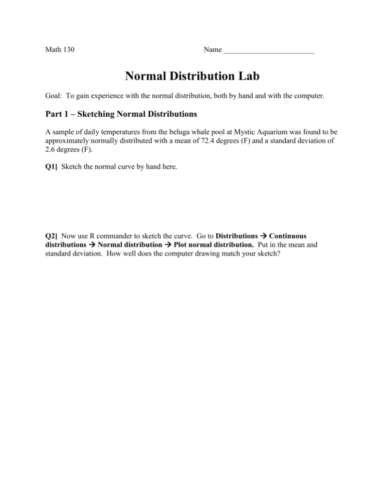
Math 130
Name ________________________
Normal Distribution Lab
Goal: To gain experience with the normal distribution, both by hand and with the computer.
Part 1 – Sketching Normal Distributions
A sample of daily temperatures from the beluga whale pool at Mystic Aquarium was found to be
approximately normally distributed with a mean of 72.4 degrees (F) and a standard deviation of
2.6 degrees (F).
Q1] Sketch the normal curve by hand here.
Q2] Now use R commander to sketch the curve. Go to Distributions  Continuous
distributions  Normal distribution  Plot normal distribution. Put in the mean and
standard deviation. How well does the computer drawing match your sketch?
Using a normal model, we are often interested in the percentage of observations in a certain
range. For example, we might be interested in the percentage of days where the temperature is
above 75 degrees.
Normal percentages can be pictured as shaded areas under the normal curve as shown below.
1
−
1
(𝑦−𝜇)2
The normal curve has a formula: √2𝜋𝜎2 𝑒 2𝜎2
. The area is formally computed by
integrating the area under this curve, but that is not trivial. It has to be done numerically.
There are several ways to go about this:
 Use an approximation with the 68-95-99.7 rule
 Use a more exact hand calculation with a Z-table
 Use a statistics software package
Part 2 – Using the 68-95-99.7 rule
A rule of thumb for normal distributions is the following:
 Approximately 68% of observations are within 1 standard deviation of the mean
 Approximately 95% of observations are within 2 standard deviations of the mean
 Approximately 99.7% of observations are within 3 standard deviations of the mean
We then know that 68% of the observations are between 69.8 and 75 degrees. This leaves 32%
left over, or 16% below 69.8 degrees and 16% above 75 degrees.
Use the 68-95-99.7 rule to approximate the following percentages:
Q3] The percentage of days less than 67.2 degrees.
Q4] The percentage of days greater than 69.8 degrees.
Part 3 – Using the Z-table
Suppose instead that we wanted to find the percentage of days with a temperature over 76
degrees. We have a problem here, as 76 is not a multiple of the standard deviation. Using the
68-95-99.7 rule, we can only guess that the percentage of days is between 16% and 2.5%, not
very helpful.
A more accurate way to get this percentage is to look it up on a table of areas that are computed.
However, we’d need a separate table for each different normal distribution. To get around this
there is a table in your book that is created for the standard normal distribution, with a mean of
zero and a standard deviation of 1.
So, we are trying to find the area above 76 degrees. To do this, we convert to a standard normal
𝑦−𝜇
76−72.4
using the Z-score: 𝑍 = 𝜎 = 2.6 = 1.38. The area above 76 degrees is the same as the area
above 1.38 for a standard normal variable.
The Z-table (attached at the end of this lab) give the area to the left of 1.38. Look up 1.38 in the
table, and we find that the area to the left of 1.38 is 0.9162. This leaves a percentage of 0.0838
to the right.
Answer: 8.38% of days have a temperature above 76 degrees.
Q5] Now it’s your turn. Approximately what percentage of the time are the temperatures in the
pool:
a. Greater than 78 degrees?
b. Below 70 degrees?
c. Between 60 and 70 degrees?
Part 4 – Using R Commander
The Rcmdr software package will compute normal probabilities as well. Let’s reconsider the
example above, where the mean is 72.4, the standard deviation is 2.6, and we’re interested in
the percentage of days above 76 degrees.
Go to Distributions  Continuous distributions  Normal distribution  Normal
probabilities. Plug in the y value soon, along with the mean and standard deviation. If you
want the percentage below 75 degrees, select the “lower tale” radio button. If you want the
percentage above 75 degrees, use the “upper tale” radio button.
We find that the percentage is 0.0831, similar to what we found by hand in Part 3 of this lab.
Q6] Redo the parts of Q5 using R commander.
Part 5 – Normal Percentiles
The previous work of this lab gave us an observation value and asked for a percentage related
to it. Example: What percentage of days would we expect to have a temperature of over 76
degrees?
We can also do the reverse, and ask for the observation value that has a given percentage of
observations above or below it. For example: Above what temperature are the hottest 15%
of recordings?
This number is sometimes referred to as the 85th percentile. The pth percentile is a value
with p% of the data below it.
By Hand: We begin by using the Z-table. We seek the Z value with 85% of observations
below it. Look in the body of the table to get as closest to 0.85 as we can.
The closest we get is 0.8508, corresponding to Z = 1.04. However, this is in terms of Z, not
our original y’s. To get back on our original scale, we need to transform from the Z back to
our original data:
𝑍=
1.04 =
𝑦−𝜇
𝜎
𝑦 − 72.4
2.6
𝑦 = 75.104.
Fifteen percent of the days have a temperature of 75.1 or more.
In R commander:
This is much easier in R commander. Go to Distributions  Continuous distributions 
Normal distribution  Normal quantiles. Put in the percentage of interest (below or
above), mean, standard deviation, and then select lower-tail or upper-tail depending on
whether you put in the percent below or the percent above. Then click OK.
We get 75.09473, very similar to the result we got by hand.
Q7] Below which temperature are the lowest 10% of recordings?
Part 6 – Assessing Normality
Many times we will be taking data and asserting that they are normal or approximately normal.
We’ll need to verify the normality of our data. There are several ways to do this.
First, you could do a histogram of the data, and look for a bell-shaped histogram. Next, you
could produce a normal Q-Q plot. Go to Graphs  Quantile comparison plot. If the data are
normal, they should ideally follow a straight line.
Q8] Create a histogram and normal Q-Q plot of our classroom height data. What do you find?