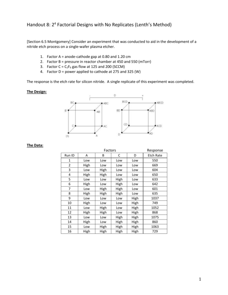
Handout 8: 24 Factorial Designs with No Replicates (Lenth’s Method)
[Section 6.5 Montgomery] Consider an experiment that was conducted to aid in the development of a
nitride etch process on a single-wafer plasma etcher.
1.
2.
3.
4.
Factor A = anode-cathode gap at 0.80 and 1.20 cm
Factor B = pressure in reactor chamber at 450 and 550 (mTorr)
Factor C = C2F6 gas flow at 125 and 200 (SCCM)
Factor D = power applied to cathode at 275 and 325 (W)
The response is the etch rate for silicon nitride. A single replicate of this experiment was completed.
The Design:
The Data:
Factors
Run ID
1
2
3
4
5
6
7
8
9
10
11
12
13
14
15
16
A
Low
High
Low
High
Low
High
Low
High
Low
High
Low
High
Low
High
Low
High
B
Low
Low
High
High
Low
Low
High
High
Low
Low
High
High
Low
Low
High
High
C
Low
Low
Low
Low
High
High
High
High
Low
Low
Low
Low
High
High
High
High
Response
D
Low
Low
Low
Low
Low
Low
Low
Low
High
High
High
High
High
High
High
High
Etch Rate
550
669
604
650
633
642
601
635
1037
749
1052
868
1075
860
1063
729
1
The Data in Minitab (EtchRate.MPJ)
Coded Effects
Uncoded Effects
2
The Analysis
Under the Terms… tab, specify all factors to be included in our analysis…
How many terms are in this model? How many design points do we have?
Realize, this is an unreplicated design with no center runs…
3
Once again, all residuals are zero and so an independent estimate of error cannot be obtained.
This experiment is void of center runs which are what “saved us” on the last handout.
The output from Minitab is incomplete and does not provide a statistical test that can be used
to identify significant factors.
4
The alternative approach of using a Normal Probability Plot is possible in Minitab.
Minitab needed to obtain an estimate of experimental error before this plot could be created.
Minitab used Lenth’s PSE method to obtain this estimate of error. See page 237 of textbook for
Lenth’s procedure.
How does Minitab draw it’s blue line?
Normal probability plot
The method Minitab uses to draw the normal effects plot depends on the degrees of freedom for the error term.
If the error term has one or more degrees of freedom, Minitab plots the normal scores, probabilities or percentages versus the
standardized effects. The line passes through the origin (or 0.50, 0 if probabilities or percentages are used) and has a slope of
one because this is where the points are expected to lie if all effects are zero. Effects with p-values less than alpha are labeled
significant on the graph. Minitab labels this graph Normal Probability Plot of the Standardized Effects.
If the error term has zero degrees of freedom, Minitab plots the normal scores, probabilities or percentages versus the
nonstandardized effects. The line passes through the origin (or 0.50, 0 if probabilities or percentages are used) and the slope is
1/ Lenth's pseudo standard error. Effects with an absolute value exceeding the margin of error (ME) are labeled significant on
the plot. Margin of error is:
ME = t*PSE
where t is the (1 - a / 2) quantile of a t-distribution with degrees of freedom equal to the (number of effects / 3). Minitab labels
this graph Normal Probability Plot of the Effects.
For more information on how Minitab calculates PSE, see Lenth's pseudo standard error.
5
Obtaining Lenth’s Pseudo Standard Error (PSE)
The following procedure is used to compute Lenth’s pseudo standard error (PSE).
Step 1: Calculate s0
𝑠0 = 1.5 ∗ 𝑚𝑒𝑑𝑖𝑎𝑛( |𝐸𝑠𝑡𝑖𝑚𝑎𝑡𝑒𝑑 𝐸𝑓𝑓𝑒𝑐𝑡| )
Step 2: Calculate the pseudo standard error (PSE)
𝑃𝑆𝐸 = 1.5 ∗ 𝑚𝑒𝑑𝑖𝑎𝑛(|𝐸𝑠𝑡𝑖𝑚𝑎𝑡𝑒𝑑 𝐸𝑓𝑓𝑒𝑐𝑡| ∶ |𝐸𝑠𝑡𝑖𝑚𝑎𝑡𝑒𝑑 𝐸𝑓𝑓𝑒𝑐𝑡| < 2.5 ∗ 𝑠0 )
Identification of Significant Effects
After a pseudo standard error is obtained, Lenth’s approach is similar to our standard approach. A test
statistic is computed for each effect as follows.
𝑇𝑒𝑠𝑡 𝑆𝑡𝑎𝑡𝑖𝑠𝑡𝑖𝑐 =
Version
|𝐸𝑠𝑡𝑖𝑚𝑎𝑡𝑒𝑑 𝐸𝑓𝑓𝑒𝑐𝑡| − 0
𝑃𝑆𝐸
T-Distribution
T – Cutoff value
Version #1
When interest lies in
only a single effect
𝑡(𝑝𝑟𝑜𝑏 = 𝛼⁄2 , 𝑑𝑓 = 𝑚⁄3)
where
𝛼 = 0.05
𝑚 = 2𝑘 − 1
Excel: =TINV(0.025,5)
Version #2
When interest lies in
all effects
𝑡(𝑝𝑟𝑜𝑏 = 𝛾, 𝑑𝑓 = 𝑚⁄3)
where
𝛾 = 1 − ((1 + (1 − 𝛼)1/𝑚 )/2)
𝑚 = 2𝑘 − 1
Excel: =TINV(0.0017,5)
Lenth’s Decision Rule
Testing a Single Effect
Approach
Test Statistic
𝑇𝑒𝑠𝑡 𝑆𝑡𝑎𝑡𝑖𝑠𝑡𝑖𝑐 > 𝑡(𝑝𝑟𝑜𝑏 = 𝛼⁄2 , 𝑑𝑓 = 𝑚⁄3)
Testing All Effects
𝑇𝑒𝑠𝑡 𝑆𝑡𝑎𝑡𝑖𝑠𝑡𝑖𝑐 > 𝑡(𝑝𝑟𝑜𝑏 = 𝛾, 𝑑𝑓 = 𝑚⁄3)
P-Value
𝑝 − 𝑣𝑎𝑙𝑢𝑒 < 𝛼
𝑝 − 𝑣𝑎𝑙𝑢𝑒 < 𝛾
A margin-of –error concept can also be obtained via Lenth’s procedure. Two forms exist based on which
version from above is of interest.

𝑀𝑎𝑟𝑔𝑖𝑛 𝑜𝑓 𝐸𝑟𝑟𝑜𝑟 = 𝑡(𝑝𝑟𝑜𝑏 = 𝛼⁄2 , 𝑑𝑓 = 𝑚⁄3) ∗ 𝑃𝑆𝐸

𝑆𝑖𝑚𝑢𝑙𝑡𝑎𝑛𝑒𝑜𝑢𝑠 𝑀𝑎𝑟𝑔𝑖𝑛 𝑜𝑓 𝐸𝑟𝑟𝑜𝑟 = 𝑡(𝑝𝑟𝑜𝑏 = 𝛾, 𝑑𝑓 = 𝑚⁄3) ∗ 𝑃𝑆𝐸
6
Doing the computations in Excel
The computations for Lenth’s procedure as shown here for our example.
Notice the PSE here matches Minitab’s Lenth PSE reported on the Normal Quantile Plot:
7
The Test Statistics can be computed directly in Excel once an estimate of the standard error is obtained.
The =TINV() function in Excel can be used to obtain the T-Cutoff values discussed above. The test
statistics can be compared directly against these value.

Version #1: =TINV(0.025,5)

Version #2: =TINV(0.0017,5)
8
The p-value approach is preferred. The =TDIST() function can be used in Excel to obtain a p-value for
each effect. Realize, the bottom-up approach should be used in the evaluation of significant effects.
The “2” in the TIDST() function specifies a two-tailed test which is the desired test, i.e. just need an
effect away from 0.
=TDIST( Test Statistic, df = m/3, 2)

Version #1: Compare p-value against 

Version #2: Compare p-value against 
Questions:
1. What are the significant effects using a standard error rate of 0.05?
2. What are the significant effects using gamma?
3. Discuss the similarities and/or differences…
9
A quick look at plots…
Note, proceed with caution in looking at these plots as the 4-way interaction is important in this
example.
10
11