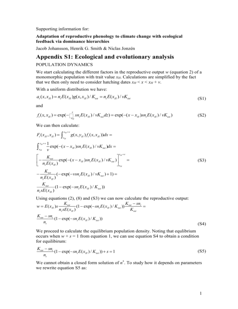
Supporting information for:
Adaptation of reproductive phenology to climate change with ecological
feedback via dominance hierarchies
Jacob Johansson, Henrik G. Smith & Niclas Jonzén
Appendix S1: Ecological and evolutionary analysis
POPULATION DYNAMICS
We start calculating the different factors in the reproductive output w (equation 2) of a
monomorphic population with trait value xH. Calculations are simplified by the fact
that we then only need to consider hatching dates xH < x < xH + v.
With a uniform distribution we have:
at (x, xH ) = nt E(xH )g(x, xH ) / Ktot = nt E(xH ) / vKtot
(S1)
and
x
ft (x, xH ) = exp(- ò snt E(xH ) / vKtot dz) = exp(-(x - xH )snt E(xH ) / vKtot )
xH
(S2)
We can then calculate:
Ft (x H , xH ) = ò
ò
x H +v
xH
x H +v
xH
g(x, yH ) ft (x, x H ))dx =
1
exp(-(x - x H )snt E(xH ) / vK tot )dx =
v
x H +v
é
ù
K tot
ê - n E(x ) exp(-(x - x H )snt E(x H ) / vK tot ) ú
ë t
û xH
H
=
(S3)
K tot
(- exp(-vsnt E(x H ) / vK tot ) + 1) =
nt E(x H )
K tot
(1- exp(-snt E(x H ) / K tot ))
nt sE(xH )
-
Using equations (2), (8) and (S3) we can now calculate the reproductive output:
K tot
K - snt
w = E(xH )s
(1- exp(-snt E(xH ) / K tot )) tot
=
nt sE(xH )
K tot
K tot - snt
(1- exp(-snt E(xH ) / K tot ))
nt
(S4)
We proceed to calculate the equilibrium population density. Noting that equlibrium
occurs when w + s = 1 from equation 1, we can use equation S4 to obtain a condition
for equilibirum:
K tot - snt
(1- exp(-snt E(xH ) / K tot )) + s = 1
nt
(S5)
We cannot obtain a closed form solution of n*. To study how it depends on parameters
we rewrite equation S5 as:
1
(1- exp(-snt E(xH ) / K tot )) =
1- s
nt
Ktot - snt
(S6)
With regard to the left hand side (LHS) of equation S6 we note that 1 - exp(-y) is an
increasing and decelerating function of y. It follows that LHS increases with s, n, E
and decreases with Ktot. The right hand side (RHS) of equation S6 increases with n
and is furthermore an accelerating function of n. It decreases with Ktot. Since n < Ktot
the nominator decreases more with s than the denominator. The RHS hence decreases
with s.
Since LHS is a decelerating function and RHS is a accelerating function, LHS > RHS
for n < n*. Therefore increasing LHS for all values of n, increases n*. Likewise
decreasing RHS for all values of n, also increases n*. LHS decreases with E and RHS
is independent of E. It follows that n* increases with E. LHS increases with s and RHS
decreases with s and it therefore follows that n* increases with s as well.
Finally we calculate the minimal values of E and s for the population to be able to
grow at all. We thus consider the conditions for per capita growth being above 1 when
the population density goes to zero. The per capita growth rate in our model is w + s .
If we let n go to zero, it affects w but not s. Using l'Hopitals rule we see that:
K tot - sn
nsE(xH )
(1- exp()) =
n®0
n
K tot
lim w = lim
n®0
DK tot (1- exp(-
K tot
nsE(xH )
(1- exp()) = lim
n®0
n
K tot
sE(xH )
nsE(xH )
K tot
exp())
K tot
K tot
lim
= sE(xH )
n®0
1
lim
n®0
Dn
nsE(x H )
))
K tot
=
(S7)
The per capita growth when n goes to 0 is hence equal to sE + s. Therefore we
conclude that for postive growth at low densities it is necessary that
sE + s > 1.
(S8)
An interpretation of this condition is that the adult needs to replace itself, either by
producing an offspring that survives (which occurs with probability sE) by surviving
itself (which occurs with probability s).
2
EVOLUTIONARY ANALYSIS
Selection gradient
We here explain how we derived the selection gradient (equation 12). Writing out
equation (1) using equations (3), (7) and (8) we obtain:
w(yH , xH ) = E(yH )s
Ktot - sn*
F(yH , xH )
Ktot
(S9)
F depends on f which in the interval xH < x < xH + v amounts to:
f (x, xH ) = exp(- ò
x
xH
sn*E(xH )
/ Ktot dz)
v
(S10)
We will use this to calculate F explictly. If yH > xH we get:
¥
F(yH , xH ) = ò g(x, yH ) ft (x, x H ))dx =
yH
ò
x H +v
yH
yH +v 1
1
x - x H n*sE(xH )
n*sE(x H )
exp()dx + ò
exp()dx =
x H +v v
v
v
K tot
K tot
x H +v
(S11)
é
K tot
x - xH n*E(xH ) ù
yH - x H
n* sE(xH )
)ú
+
exp()=
ê - n* sE(x ) exp(- v
K tot
v
K tot
ë
û yH
H
K tot é
yH - xH n* sE(xH )
n*sE(xH ) ù yH - xH
n* sE(xH )
exp()
exp()
+
exp()
ú
n*sE(xH ) êë
v
K tot
K tot
v
K tot
û
If yH < xH we then get
F(yH , x H ) = ò
xH
yH
yH +v 1
1
x - xH n*sE(xH )
dx + ò
exp()dx =
xH
v
v
v
K tot
yH +v
x H - yH é
K v
x - xH n*sE(xH ) ù
+ ê - * tot
exp()ú
v
v
K tot
ë n svE(xH )
û xH
=
(S12)
x H - yH
K tot é
yH + v - xH n*sE(xH ) ù
+ *
1- exp()ú
v
n sE(xH ) êë
v
K tot
û
In order to obtain the selection gradient we will need the derivative:
S(xH ) =
¶w(yH , xH ) + s
¶yH
yH =xH
=
¶w(yH , xH )
¶yH
yH =xH
(S13)
As a preparatory step we calculate:
¶w(yH , xH )
K - sn*
¶F(yH , yH )
= s tot *
(E '(yH )F(yH , yH ) + E(yH )
)
¶yH
n
¶yH
(S14)
Next we calculate the different components from equation S8 that we still do not
have. We note that:
E '(yH ) =
xopt - yH
s
2
E0 exp(-(yH - xopt )2 / 2s 2 ) =
xopt - yH
s2
E(yH ) .
(S15)
3
We then calculate the derivatives of F, for yH > xH we get:
¶F(yH , xH )
=
¶yH
1 n* sE(xH ) K tot v é
yH - xH n*sE(x H ) ù 1
n* sE(xH )
exp() ú + exp()=
v K tot n*sE(x H ) êë
v
K tot
K tot
û v
1é
y - xH n* sE(xH ) ù 1
n*sE(x H )
- ê exp(- H
) ú + exp()
vë
v
K tot
K tot
û v
(S16)
For yH < xH we get:
¶F(yH , xH )
=
¶yH
1 1 n*sE(xH ) K tot é
yH + v - x H n*sE(xH ) ù
- +
exp()ú =
v v K tot n*sE(xH ) êë
v
K tot
û
(S17)
1 1é
y + v - xH n*sE(xH ) ù
- + êexp(- H
)ú
v vë
v
K tot
û
Since we are interested in the selection gradient when yH = xH , we will evaluate the
different components there as a preparatory step. F(xH, xH) is given from equation S11
above when substituting nt for n*. Evaluating the respective derivatives at yH = xH in
both cases gives:
¶F(yH , xH )
¶yH
yH =xH
ù
1 1é
n*sE(xH ) ù 1 é
n*sE(xH )
= - + êexp()ú = êexp() -1ú
v vë
Ktot
Ktot
û vë
û
(S18)
Due to the similarity with F in equation S3 we write this derivative as:
¶F(yH , xH )
¶yH
yH =x H
=-
n*sE(xH )
F(xH , xH )
Ktot
(S19)
Finally we put the pieces together:
¶w(yH , x H )
¶yH
s
yH =xH
=
K tot - sn* xopt - xH
n*sE 2 (xH )
(
E(x
)F(x
,
x
)
F(xH , xH )) =
H
H
H
K tot
s2
vK tot
E(xH )s
(S20)
x -x
K tot - sn*
n*sE(xH )
F(xH , xH )( opt 2 H )
K tot
s
vK tot
The first four factors in the expression can be identified as reproductive output w (cf.
equation S1). At population dynamical equilibrium we further have w = 1 - s. Hence
we have the following are equivalent expressions for the selection gradient (equation
12):
S(xH ) = w(xH , xH )(
xopt - xH
s2
-
x -x
n*sE(xH )
n*sE(xH )
) = (1- s)( opt 2 H )
vK tot
s
vK tot
(S21)
4
Convergence stability
Conforming to notation in the main text we express the selection gradient as
S(xH ) = (1- s)[L(xH ) - R(xH )]
(S22)
As explained in the main text the singular point x H* is found when L(xH) = R(xH). As
shown in Fig. 3b, L decreases with xH and R is a positive number with a maximum at
xH = 0. It follows that xH* < 0 . When the resident has a trait value xH < xH* we also
see that L(xH) > R(xH) since L increases and R decreases when the value of xH is below
x H* and decreases. In such situations, there is hence selection for higher values of xH.
Following a similar reasoning, we see that a similar reasoning shows that there is
selection for lower values of xH when the resident a trait value xH > xH* . We conclude
that gradual evolution will lead to x H* regardless of starting point, and thus x H* is
convergence stable (Geritz et al. 1998).
Resistance to invasions
We studied invasion resistance of singular points numerically. We evaluated equation
10 for invading traits yH in the interval xH* -1 < yH < xH* +1 for the parameter
combinations shown in Fig. 4. In all cases the singular points corresponded to the
maximum of the invasion fitness, and hence were resistant to invasion (Geritz et al.
1998).
5