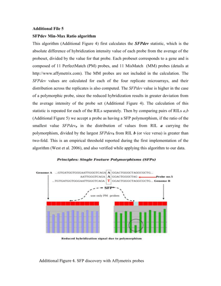
Additional File 5
SFPdev Min-Max Ratio algorithm
This algorithm (Additional Figure 4) first calculates the SFPdev statistic, which is the
absolute difference of hybridization intensity value of each probe from the average of the
probeset, divided by the value for that probe. Each probeset corresponds to a gene and is
composed of 11 PerfectMatch (PM) probes, and 11 MisMatch (MM) probes (details at
http://www.affymetrix.com). The MM probes are not included in the calculation. The
SFPdev values are calculated for each of the four replicate microarrays, and their
distribution across the replicates is also computed. The SFPdev value is higher in the case
of a polymorphic probe, since the reduced hybridization results in greater deviation from
the average intensity of the probe set (Additional Figure 4). The calculation of this
statistic is repeated for each of the RILs separately. Then by comparing pairs of RILs a,b
(Additional Figure 5) we accept a probe as having a SFP polymorphism, if the ratio of the
smallest value SFPdeva in the distribution of values from RIL a carrying the
polymorphism, divided by the largest SFPdevb from RIL b (or vice versa) is greater than
two-fold. This is an empirical threshold reported during the first implementation of the
algorithm (West et al. 2006), and also verified while applying this algorithm to our data.
Additional Figure 4. SFP discovery with Affymetrix probes
Additional Figure 5. SFPdev Min-Max Ratio algorithm
RIL Bimodal Distributions algorithm. This algorithm is similar to K-means clustering
with K = 2. In summary, the RIL Bimodal Distributions (Additional Figure 6) algorithm
first calculates the absolute values of probe intensity differences dijk (probe i, probeset j,
RIL k), from the average of each probeset. Similarly with the SFPdev, only PM probes
are included in the calculation. In the next step, the algorithm computes the distribution
of each dijk value across all the individuals of the RIL population. The median Mij is
initially used to split the distribution into an upper (u) and lower (l) subsets (Additional
Figure 7). The averages lavg , uavg of the l and u subsets respectively, are the seeding
centers for the K-means clustering. Then the algorithm iterates in the same manner for
eight times , but instead of the Mij, it uses the average (lavg + uavg)/2 for splitting again
into u,l subsets. After all iterations, the dijk values settle into a bimodal distribution, with
each mode corresponding to a K-means cluster. These steps are repeated for probes in all
the probesets, measured in the expression profile of each individual of the population. In
order to assess significant separation between the two distribution modes (or otherwise
the two clusters), we use as metric the peak separation ps = (Al – Au)/√(Sl 2/nl + Su2/nu)
(Al and Au are distribution averages for the u,l modes respectively, standard deviations Sl
and Su, sample sizes nl and nu).
The algorithm also computes the dij values (averaged across replicate microarrays) for
the PI407162 and V71-370 parental data. For polymorphic probes, dijk values for the
individuals of the RIL population are expected to cluster around the parental dij, under
the two modes of the distribution (Additional Figure 7). Since the RIL population was
created by the cross of the genetically distant PI407162 and V71-370 soybean lines, the
two modes originate due to the different parental alleles inherited to the RIL progeny. For
each SFP probe, RIL individuals are assigned a genotype based on their clustering around
one of the parental values (Additional Figure 7).
Additional Figure 6. Details of the RIL Bimodal Distributions algorithm
PI407162
V71-370
Additional Figure 7. Genotyping RILs based on parental genotypes to the bimodal distribution