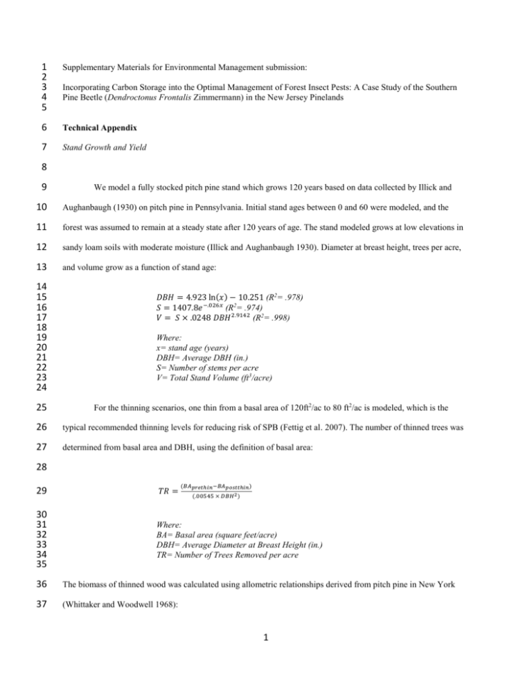
1
2
3
4
5
Supplementary Materials for Environmental Management submission:
6
Technical Appendix
7
Stand Growth and Yield
Incorporating Carbon Storage into the Optimal Management of Forest Insect Pests: A Case Study of the Southern
Pine Beetle (Dendroctonus Frontalis Zimmermann) in the New Jersey Pinelands
8
9
We model a fully stocked pitch pine stand which grows 120 years based on data collected by Illick and
10
Aughanbaugh (1930) on pitch pine in Pennsylvania. Initial stand ages between 0 and 60 were modeled, and the
11
forest was assumed to remain at a steady state after 120 years of age. The stand modeled grows at low elevations in
12
sandy loam soils with moderate moisture (Illick and Aughanbaugh 1930). Diameter at breast height, trees per acre,
13
and volume grow as a function of stand age:
14
15
16
17
18
19
20
21
22
23
24
25
𝐷𝐵𝐻 = 4.923 ln(𝑥) − 10.251 (R2= .978)
𝑆 = 1407.8𝑒 −.026𝑥 (R2= .974)
𝑉 = 𝑆 × .0248 𝐷𝐵𝐻 2.9142 (R2= .998)
Where:
x= stand age (years)
DBH= Average DBH (in.)
S= Number of stems per acre
V= Total Stand Volume (ft3/acre)
For the thinning scenarios, one thin from a basal area of 120ft2/ac to 80 ft2/ac is modeled, which is the
26
typical recommended thinning levels for reducing risk of SPB (Fettig et al. 2007). The number of thinned trees was
27
determined from basal area and DBH, using the definition of basal area:
28
(𝐵𝐴𝑝𝑟𝑒𝑡ℎ𝑖𝑛 −𝐵𝐴𝑝𝑜𝑠𝑡𝑡ℎ𝑖𝑛)
29
𝑇𝑅 =
30
31
32
33
34
35
Where:
BA= Basal area (square feet/acre)
DBH= Average Diameter at Breast Height (in.)
TR= Number of Trees Removed per acre
(.00545 × 𝐷𝐵𝐻 2 )
36
The biomass of thinned wood was calculated using allometric relationships derived from pitch pine in New York
37
(Whittaker and Woodwell 1968):
1
38
39
40
41
42
43
44
45
𝑂𝐷𝐵 = ( .1040𝐷𝐵𝐻 2.3373 ) × 𝑇𝑅
Where:
ODB= Oven Dry Above-ground Biomass (kg/acre)
DBH= Diameter at breast height (cm)
TR= Number of Trees removed per Acre
46
Basal area and thus the weighted incidence probabilities are recalculated after thinning using growth and
47
yield relationships. Because the effects of thinning on growth rates of remaining trees in pitch pine stands in New
48
Jersey has not been studied, DBH growth rates of trees are adjusted to increase .01 in. per year after thinning. This
49
estimate was based on the range of increased growth rates from data of shortleaf and loblolly stands in the South
50
(Feduccia et al. 1979; Mann 1952).
51
52
Southern Pine Beetle Infestations and Ecological Data
53
54
55
This study considers a weighted incidence probability used in previous literature, as well as regional SPB
population levels and climate to stochastically generate SPB infestations through Monte Carlo simulations.
56
57
Weighted Incidence Probability: We consider a model in which the risk of a Southern Pine Beetle attack increases
58
as a function of basal area of a stand, according to the Daniel’s (1979) incidence probability function:
59
60
61
1
𝑃𝐷𝐾 =
1 + 𝐸𝑋𝑃(4.829 − (. 0519 ∗ (
62
63
64
65
66
67
(
𝐵𝐴
)) − (4.062 ∗ (%𝑃𝑆𝐶))
4.356
)
Where:
PDK= Daniels Incidence Probability for stand
BA= Basal area (m2/ac)
%PSC= Percent pine composition of stand
68
This incidence probability has been used in previous models of SPB pestilence (Costanza et al. 2012; Burkhart et al.
69
1986). Percent pine composition of the stand is assumed to be a constant 80% as in Reed et al. (1982).
70
71
The Daniels function estimate is “unweighted,” or it assumes that there are an equal number of infested and
un-infested stands in a region. Thus, it must be adjusted for region-wide infestation risk or the average number of
2
72
infested stands of host type across the region during an outbreak year. In order to weight this function, we use a
73
similar weighting system as Naumann (2012) to adjust the Daniels et al. (1979) probability function by the New
74
Jersey regional risk:
75
𝑃𝑠
𝑃̅𝐷
76
𝑃𝑘 = 𝑃𝐷𝑘 ∗
77
78
79
80
81
82
83
Where:
Pk = probability of mortality from SPB
Ps= regional SPB risk
PDk= Daniels probability
𝑃̅𝐷 = average Daniels probability for stand
84
New Jersey regional SPB risk was determined through an ArcGIS analysis of New Jersey Department of
85
Environmental Protection SPB spot data between 2002 and 2011 over outbreak years and New Jersey Department of
86
Environmental Protection Land Use Land Cover (LULC) 2007 data on forest types. Stands were assumed to have
87
similar species composition between 2002-2011 as they had when they were surveyed in 2007. The regional SPB
88
risk, measured in median infested acres/ acre of host type for outbreak years, was calculated assuming that any
89
stands with greater than 50% conifer composition were host stands.
90
91
Regional SPB Populations: In this model, each year was stochastically determined to be an “outbreak year,” in
92
which the weighted incidence probability was invoked, or an “endemic year,” in which SPB populations were
93
assumed to be so low that no forest damage occurred. In endemic years, the weighted incidence probability was
94
assumed to be 0. We modeled high, medium, and low SPB population levels, in which 80%, 50%, and 20% of years
95
modeled, respectively, were outbreak years.
96
97
Climate: Climate, another factor that is not typically incorporated into economic analyses of SPB infestations, is
98
also incorporated into this model for greater biological accuracy. Studies have projected that future climate change
99
may increase SPB infestation risk in certain areas by 2.5-5 times (Gan, 2004). Minimum winter temperature (MWT)
100
was modeled in this study because it is the most well-known regulating factor of SPB outbreak, since notable winter
101
mortality occurs when temperatures drop below -12°C and beetles freeze (Lombardero et al. 2000a). Tran et al.
3
102
(2007) found that if the coldest winter night dropped below -16°C, the probability of a decrease in SPB population
103
was 65%. If temperatures dropped below -20°C, then there was an 80% likelihood that populations significantly
104
declined. This study thus assumed the same criteria as Tran et al. (2007).
105
106
Volumetric Losses and Severity: If a stand is determined to be infested based on the incidence probability, climate,
107
and regional outbreak, we assume that a “spot” or growing infestation will develop that affects a proportion of the
108
stand. We assume that suppression will stop spot growth after 45 days (Burkhart et al. 1986) while no management
109
will allow spot growth to continue throughout the summer (Fettig et al. 2007), which we modeled as being 120 days.
110
Many studies of SPB in the South have documented that spot growth and thus volumetric losses from SPB vary with
111
basal area, DBH and other stand parameters (Lorio et al. 1982; Nebeker et al. 1985). Thus, we used the Reed et al.
112
(1981) severity function derived from data in Texas to model spot growth over the 45 or 120 day period of spot
113
growth:
𝑇𝐵𝐴
𝑙𝑛(𝑇𝐾𝐷) = 3.43 + .965𝑙𝑛(𝐴𝑇) − 2.85𝑙𝑛(𝐷𝐵𝐻) − 22.13(
) + .074𝑇𝐵𝐴 + .5576𝑃𝑂𝑃
𝐷𝐵𝐻 2
114
115
116
117
118
119
120
121
122
123
As in Burkhart et al. (1986) we assume the initial spot size is .05 acres so the number of initial attacked trees is
124
derived from stand density at the time of infestation. Volumetric losses are then calculated using the following
125
formula, based on Burkhart et al. (1986) and pitch pine growth and yield from Illick and Aughenbaugh (1930):
126
Where:
TKD= Trees killed per day
AT=Number of initial attacked trees
DBH= Diameter at breast height (cm)
TBA= Total Basal Area (m2/ha)
POP= annual number of spots/405 ha of host trees for entire region/year
𝑉𝐿 = (𝐴𝑇 + (𝑇𝐾𝐷 ∗ 𝐷)) ∗ .0248 ∗ (𝐷𝐵𝐻 2.9143 )
Where:
TKD= Trees killed per day
AT=Number of initial attacked trees
DBH= Diameter at breast height (cm)
D= Days of spot growth
127
128
129
130
131
132
133
Once volumetric losses are calculated, the proportion of the stand infested, or the “sub-stand” is reset to stand age of
134
zero while the remaining proportion of the stand continues growing unharmed. Basal areas and thus infestation
135
probabilities are then weighted based on the proportion of the stand each “sub-stand” represents. We assume our
136
stand is infested a maximum of seven times in the 120 year modeling period.
4
137
138
Incorporating and Valuing Carbon Sequestration
139
140
Following Gutrich and Howarth’s (2007) model, carbon storage is determined from four main components:
141
live above ground biomass, root biomass, soil, and dead and downed wood. Carbon is then valued assuming a future
142
global carbon emissions and offsets trading market, as in Gutrich and Howarth (2007), and incorporated into
143
economic analyses using social net present value calculations.
144
145
Live Biomass: Carbon in live biomass is calculated from total above and below ground biomass of trees using the
146
50% rule, which is the default used in IPCC reports. This rule states that standing live carbon content of a stand is
147
approximately 50% of oven-dry biomass ( Brown and Lugo 1982). As was followed in Lathrop et al.’s (2011)
148
analysis of carbon sequestration in New Jersey, below ground, or root biomass, was assumed to be directly related to
149
above ground biomass, using relationships developed by Cairns et al. (1997):
150
151
𝑅𝐵 = 𝐸𝑋𝑃(−1.085 + .926𝐿𝑛(𝐴𝐺𝐵))
152
153
154
155
156
where:
RB= Root Biomass (tons/acre)
AGB= Above ground Biomass (tons/acre)
157
Soil Carbon: Soil carbon was assumed to be independent of management as in Gutrich and Howarth (2007) and thus
158
assumed to be a constant value of 20 tons/acre in this study. This figure was derived from Lathrop et al. (2011), who
159
found from USDA Soil Survey Geographic (SSURGO) database and Forest Inventory and Analysis data that soil
160
carbon density in the Pinelands ranged from between 20 and 75 tons/ acre. The highest soil carbon densities were
161
found in poorly drained soils of coastal wetland areas, while the lowest soil carbon densities were found in the drier
162
soils of the Uplands, which most closely resembled the soil conditions of the stands modeled in Illick and
163
Aughanbaugh (1930).
164
5
165
Dead and Downed Wood: Carbon in dead and downed wood was determined from an equation developed by
166
Gutrich and Howarth (2007), which allows dead and downed wood to decay at a certain rate each year and new dead
167
biomass to be added each year to the dead and downed wood stock:
168
169
170
171
172
173
174
175
𝐶𝑑𝑒𝑎𝑑 = (1 − 𝜕0 )[𝐶𝑑𝑒𝑎𝑑 (𝑡 − 1) + 𝜕1 𝐶𝑙𝑖𝑣𝑒 (𝑡 − 1)𝜕2 ]
where:
𝐶𝑑𝑒𝑎𝑑 = Carbon in dead/ downed wood (tons)
𝜕0 = Decay rate of dead/downed wood (%/year)
𝜕1 , 𝜕2 =Formation coefficients for dead/ downed wood
176
Formation and decay rates of dead and downed wood determined by Gutrich and Howarth from Forest Inventory
177
and Analysis data for red/white/jack pine in the Northeast were used, as no data existed for pitch pine in New Jersey.
178
It was assumed that carbon converted into mulch from thinning or cut and remove suppression was completely
179
released within a year after mulching, and trees left from cut and leave suppression were added as dead and downed
180
wood and decayed at the same rate as other dead and downed wood.
181
182
Carbon Valuation: As discussed in the manuscript, increasingly, the social costs of carbon- and thus the value of
183
carbon sequestration- are increasingly being considered in forest management. The value of carbon, or the marginal
184
benefit of a ton of carbon sequestered, can be determined from the social costs of carbon over time using an
185
Integrated Assessment Model, which uses an aggregate damage function to determine prices of carbon under future
186
emissions scenarios. We used the 2007 version of the DICE integrated assessment model (Nordhaus, 2008) to
187
determine marginal benefits over time in two potential future policy scenarios. In the first policy scenario, or the
188
“low marginal benefits of carbon scenario,” we assume climate mitigation aims to maximize net benefits and
189
marginal benefits of carbon increase over time according to the following equation:
190
191
192
193
194
195
196
𝑀𝐵𝑙𝑜𝑤 = 39.874 ∗ 𝐸𝑋𝑃(. 0167𝑡)
where:
MBlow= Marginal benefits of Carbon ($/ton)
t= time (years)
6
197
In the second policy scenario, or the “high marginal benefits of carbon” scenario, we assume emissions
198
abatement programs prevent more than a 2 degree F increase in global mean temperatures over the next century;
199
thus, marginal benefits of carbon increase over time according to the following equations:
200
201
202
203
204
205
206
207
208
For t<80,
For t>80,
𝑀𝐵ℎ𝑖𝑔ℎ = 72.987 ∗ 𝐸𝑋𝑃(.0336𝑡)
𝑀𝐵ℎ𝑖𝑔ℎ = .23267𝑡 2 − 50.217𝑡 + 3451.1
Where:
MBhigh= Marginal benefits of Carbon ($/ton)
t= time (years)
Private and Social Net Present Value Calculations:
209
210
Without considering carbon sequestration or other ecosystem services, a rational forest manager would
211
choose to follow the SPB management scenario that would maximize net benefits from chips and mulch, or the
212
private net present value:
213
214
215
216
217
218
219
220
221
222
223
224
225
120
𝑡
𝑁𝑃𝑉𝑝𝑟𝑖𝑣𝑎𝑡𝑒 = ∑(𝑅𝑡ℎ𝑖𝑛 − 𝐶𝑡ℎ𝑖𝑛 + 𝑅𝑠𝑢𝑝𝑝𝑟𝑒𝑠𝑠𝑖𝑜𝑛 − 𝐶𝑠𝑢𝑝𝑝𝑟𝑒𝑠𝑠𝑖𝑜𝑛 ) ∏
𝑡=0
𝑖=1
1
(1 + 𝑟(𝑖))
Where:
𝑅𝑡ℎ𝑖𝑛 = Revenue from 1 acre of thinning
𝐶𝑡ℎ𝑖𝑛 = Costs/acre of thinning
𝑅𝑠𝑢𝑝𝑝𝑟𝑒𝑠𝑠𝑖𝑜𝑛 = Revenue/ acre of suppression
𝐶𝑠𝑢𝑝𝑝𝑟𝑒𝑠𝑠𝑖𝑜𝑛 = Costs/acre of suppression
r(i) = discount rate
t= time (years)
The Private NPV is calculated as zero unless the basal area of the stand exceeds 120 square feet per acre
226
and the stand is thinned or if the stand is stochastically determined to be infested that year. Marginal benefits derived
227
from chips and mulch were determined from an internet search of mulch and chip prices; the majority of the
228
contractors interviewed conducting SPB management were in the business as developers and land clearers, so the
229
marginal benefits from mulch and chips derived from costs avoided from having to buy mulch and chips for
230
developments. Costs of thinning and suppression per acre were also determined from interviews with contractors in
231
NJ. Because cost estimates per acre were provided and the majority of infestations modeled were less than an acre,
232
we modeled scenarios in which costs of suppressing an infestation were 75% and 50% of costs/per acre.
7
233
234
When carbon sequestration is considered, net benefits derived from carbon, or the carbon net present value,
can be calculated from the marginal benefits of carbon from global emissions and abatement schemes:
235
120
236
𝑁𝑃𝑉𝑐𝑎𝑟𝑏𝑜𝑛 = ∑ 𝑀𝐵(𝑡) ∗ ∆𝐶(𝑡) ∏
t=0
237
238
239
240
241
242
243
𝑡
i=1
1
(1 + 𝑟(𝑖))
Where:
MB(t)= marginal benefit of a ton of carbon sequestered
∆𝐶(𝑡)=change in carbon stored (tons) from t to t+1
r(i)= discount rate
t= time (years)
In the case of a carbon emissions and offsets market, a rational forest manager would want to maximize the
244
social net present value, or the addition of the private and carbon net present values when managing for SPB
245
pestilence:
246
247
248
249
𝑁𝑃𝑉𝑠𝑜𝑐𝑖𝑎𝑙 = 𝑁𝑃𝑉𝑝𝑟𝑖𝑣𝑎𝑡𝑒 + 𝑁𝑃𝑉𝑐𝑎𝑟𝑏𝑜𝑛
Sensitivity and Scenario Analyses:
250
251
Sensitivity analyses were conducted by varying inputs parameters by 25%. In addition, sensitivity analyses
252
were conducted for 2%, 4%, 8%, and 12% discount rates and assuming that costs of suppression for each infestation
253
(which were under an acre) were 100%, 75%, and 50% the costs of suppression per acre. Formation and decay
254
coefficients of dead and downed wood as well as regional SPB risk had the greatest effect on mean Social NPV, as
255
well as regional SPB risk. Thus, scenario analyses were conducted with dead and downed wood formation and
256
decay coefficients from the literature derived from oak/pine and white/red pine. In addition, scenarios were
257
conducted by increasing regional SPB risk two, three, and six fold to assess under what conditions thinning would
258
be favored when both carbon and timber are considered.
259
At 100% the costs of suppression, the strategy that maximized Private NPV varied based on SPB
260
population levels and initial stand age. At 50% and 75% the costs of suppression per acre, thinning maximized
261
Private NPV at all stand ages in medium population levels. However, no management strategies still maximized
262
Social NPV. Formation coefficients for oak/pine did not affect optimal management results.
8
263
For every discount rate modeled, no management strategies maximized social NPV. However, for the
264
highest discount rate scenario (12%), social NPV for thinning scenarios exceeded that of suppression cut and leave
265
scenarios (Table S-1).
266
Social net present value of thinning scenarios also exceeded that of suppression only scenarios when
267
regional SPB population risk increased to six times that of current population levels or thinning completely
268
eradicated risk of SPB and regional SPB population risk increased to two times that of current levels.
269
270
271
272
Table S-1: For all discount rates, social net present value (NPV) ($/acre) is maximized for no management
273
scenarios.
Discount rate
No management
(%/year)
Suppression cut and
Thinning and cut and
leave
leave suppression
2
1244
1181
892
4
924
886
791
8
510
486
479
2
339
315
322
274
275
276
277
References
278
279
Brown S, Lugo AE (1982) The storage and production of organic matter in tropical forests and their role in the
280
global carbon cycle. Biotropica 14:161-187
281
282
Burkhart HE, Haney Jr. HL, Newberry JD, Leuschner WA, Morris CL, Reed DD (1986) Evaluation of thinning for
283
reduction of losses from southern pine beetle attack in loblolly pine stands. South J Appl Forestry 10:105-108
284
9
285
Cairns MA, Brown S, Helmer E, Baumgardner GA (1997) Root biomass allocation in the world’s upland forests.
286
Oecologia 111:1-11
287
288
Costanza J, Huler J, Koch F, Earnhardt T, McKerrow A, Dunn P, Collazo J (2012) Stimulating the effects of the
289
southern pine beetle on regional dynamics 60 years into the future. Ecol Model 244:93-103
290
291
Feduccia DP, Dell TR, Mann WF Jr, Campbell TE, Palmer BH (1979) Yields of unthinned loblolly pine plantations
292
on cutover sites in the West Gulf Region, Res. Pap. SO-148. In: U.S. Department of Agriculture, Forest Service,
293
Southern Forest Experiment Station. New Orleans, Louisiana, p 88
294
295
Fettig CJ, Klepzig KD, Billings RF, Munson AS, Nebeker TE, Negron JF, and Nowak JT (2007) The effectiveness
296
of vegetation management practices for prevention and control of bark beetle infestations in coniferous forests of the
297
western and southern United States. Forest Ecol Manag 238:24–53
298
299
Gan JB (2004) Risk and damage of southern pine beetle outbreaks under global climate change. Forest Ecol Manag
300
191:61-71
301
302
Gutrich J, Howarth R (2007) Carbon sequestration and the optimal management of New Hampshire timber stands.
303
Ecol Econ 62:441-450
304
305
Howarth RB (2001) Intertemporal social choice and climate stabilization. Int J Environ Pollut 15:386–405
306
307
Illick JS, Aughanbaugh JE (1930) Pitch pine in Pennsylvania. Pennsylvania Department of Forestry and Waters
308
Research Bulletin 2
309
310
Lathrop R G, Clough B, Cottrell A, Ehrengeld J, Felder F, Green E.J, Specca D, Vail C, Vodak, M, Xu M., Zhang Y
311
(2011) Assessing the potential for New Jersey forests to sequester carbon and contribute to greenhouse gas
10
312
emissions avoidance. Rutgers, The State University of New Jersey. http://crssa.rutgers.edu/projects/carbon/.
313
Accessed 1 July 2013
314
315
Lombardero MJ, Ayres MP, Ayres BD, Reeve JD (2000a) Cold tolerance of four species of bark beetle (Coleoptera:
316
Scolytidae) in North America. Environ Entomol 29:421–432
317
318
Lorio P L Jr., Mason GN, Autry, GL (1982) Stand risk rating for the southern pine beetle: integrating pest
319
management with forest management. J Forest 80:212-214
320
Mann WF Jr. (1952) Thirty-six years of thinning research with loblolly pine. In: Proceedings, Louisiana State
321
University first annual forestry symposium, Baton Rouge, Louisiana, pp 1-7
322
Martinson S, Ylioja T, Sullivan B, Billings R, Ayres M (2012) Alternate attractors in the population dynamics of a
323
tree-killing bark beetle. Popul Ecol 55 (1):95
324
Naumann NB (2012) An economic assessment of stand-level treatments for southern pine beetle prevention. Master
325
of Science Dissertation, North Carolina State University Forestry and Environmental Resources.
326
327
Nebeker TE, Hodges JD, Karr BK, Moehring DM (1985) Thinning practices in southern pines--with pest
328
management recommendations. USDA Forest Service Technical Bulletin 1703:1-36
329
330
Nordhaus W (2008) A question of balance: weighing the options on global warming policies. New Haven,
331
Connecticut
332
333
Reed DD, Burkhart HE, Leuschner WA (1981) A Severity Model for Southern Pine Beetle Infestations. Forest Sci
334
27: 290-296
335
336
Reed DD, Hedden RL, Daniels RF (1982) Estimating the annual probability of southern pine beetle outbreak. Forest
337
Sci 28:202-206
11
338
339
Tran JK, Ylioja T, Billings R, Régnière J, Ayres MP (2007) Impact of minimum winter temperatures on the
340
population dynamics of Dendroctonus frontalis (Coleoptera: Scolytinae). Ecol Appl 17:882-899
341
342
Whittaker R H, Woodwell GM (1968) Dimension and production relations of trees and shrubs in the Brookhaven
343
forest, New York. J Ecol 56 (1):1-25
12