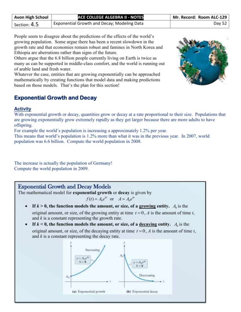
Avon High School
Section: 4.5
ACE COLLEGE ALGEBRA II - NOTES
Exponential Growth and Decay; Modeling Data
Mr. Record: Room ALC-129
Day 52
People seem to disagree about the predictions of the effects of the world’s
growing population. Some argue there has been a recent slowdown in the
growth rate and that economies remain robust and famines in North Korea and
Ethiopia are aberrations rather than signs of the future.
Others argue that the 6.8 billion people currently living on Earth is twice as
many as can be supported in middle-class comfort, and the world is running out
of arable land and fresh water.
Whatever the case, entities that are growing exponentially can be approached
mathematically by creating functions that model data and making predictions
based on those models. That’s the plan for this section!
Exponential Growth and Decay
Activity
With exponential growth or decay, quantities grow or decay at a rate proportional to their size. Populations that
are growing exponentially grow extremely rapidly as they get larger because there are more adults to have
offspring.
For example the world’s population is increasing a approximately 1.2% per year.
This means that world’s population is 1.2% more than what it was in the previous year. In 2007, world
population was 6.6 billion. Compute the world population in 2008.
The increase is actually the population of Germany!
Compute the world population in 2009.
Exponential Growth and Decay Models
The mathematical model for exponential growth or decay is given by
f (t )  A0e kt or A  A0e kt


If k > 0, the function models the amount, or size, of a growing entity. A0 is the
original amount, or size, of the growing entity at time t  0 , A is the amount of time t,
and k is a constant representing the growth rate.
If k < 0, the function models the amount, or size, of a decaying entity. A0 is the
original amount, or size, of the decaying entity at time t  0 , A is the amount of time t,
and k is a constant representing the decay rate.
Example 1
Modeling the Growth of the U.S. Population
The graph to the right shows the U.S. population, in millions,
for five selected years from 1970 through 2007. In 1970, the
U.S. population was 203.3 million. By 2007, it had grown to
300.9 million.
a. Find an exponential growth function that models the data for 1970
through 2007.
Source: U.S. Census Bureau
b. By which year will the U.S. population reach 315 million?
Our next example involves exponential decay and its use in determining the age of fossils and artifacts. The
method is based on considering the percentage of carbon-14 remaining in the fossil or artifact. Carbon-14
Decays exponentially with a half-life of approximately 5715 years. The half-life of a substance is the time
required for half of a given sample to disintegrate. Thus, after 5715 years, a given amount of carbon-14 will
have decayed to half the original amount. Carbon dating is useful for artifacts or fossils up to 80,000 years old.
Older objects do not have enough carbon-14 left to determine their age accurately.
Example 2
Carbon-14 Dating: The Dead Sea Scrolls
a. Use the fact that after 5715 years a given amount of carbon-14 will have decayed to half the original amount
to find the exponential decay model for carbon-14.
b. In 1947, earthenware jars containing what are known as the Dead Sea Scrolls were found by an Arab
Bedouin herdsman. Analysis indicated that the scroll wrappings contained 76% of their original carbon-14.
Estimate the age of the Dead Sea Scrolls.
Logisitic Growth Models
From population growth to the spread of an epidemic, nothing on Earth
can grow exponentially indefinitely. Growth is always limited. This is
shown in the figure to the right by the horizontal asymptote. The logistic
growth model is a function used to model situations of this type.
Logistic Growth Model
The mathematical model for limited logistic growth is given by
c
c
f (t ) 
or A 
,
 bt
1  ae
1  ae  bt
where a, b, and c are constants, with c  0 and b  0 .
Example 3
Modeling the Spread of the Flu
The function
30, 000
1  2e 1.5t
Describes the number of people, f (t ) , who have become ill with influenza t weeks after its initial outbreak in a
town with 30,000 inhabitants.
f (t ) 
a. How many people become ill with the flu when the outbreak began?
b. How many people were ill by the end of the fourth week?
c. What is the limiting size of f (t ) , the population that becomes ill?
Modeling Data
Throughout this chapter, we have been working with models that were given to us. However, we can create
functions that model data by observing patterns in scatter plots. The figure below shows scatter plots for data
that are exponential or logarithmic.
Choosing a Model for Data
Example 4
The bar graph in the figure to the right indicates that for the period from
2002 to 2006, an increasing number of Americans had weight-loss
surgery.
a. Create a scatter plot for the data described in the bar graph.
Use an appropriate scale.
y
x
b. What type of function would be a good choice for modeling the data? Using a graphing calculator, find a
regression equation that models the data.
c. With any regression equation, we can find a correlation coefficient. A correlation coefficient, called r, is a
value that lies between -1 and 1. A positive r in indicates a growth model, whereas a negative r indicates
decay. The closer r is to -1 or 1, the better the model fits the data. Find r for your model from part b.
Choosing a Model for Data
Example 5
It’s a new dawn for technology, appealing to people who have just hung
that huge plasma in the home theatre: the era of high-definition television.
The table shows the percentage of households in the United States with
HDTV sets for four selected years from 2001 through 2009.
a. Create a scatter plot for the data described in the bar graph.
Use an appropriate scale.
y
x
b. What type of function would be a good choice for modeling the data? Using a graphing calculator, find a
regression equation that models the data.
c. Find r for your model from part b.
Expressing an Exponential Model in Base e
y  ab x is equivalent to y  ae(ln b )x
Example 6
Rewriting the Model for World Population in Base e
The function
g ( x)  2.569(1.017) x
models world population, g ( x ) , in billions, x years after 1949. Rewrite the model in terms of base e.
What problems would we encounter from using this new model to predict future population?