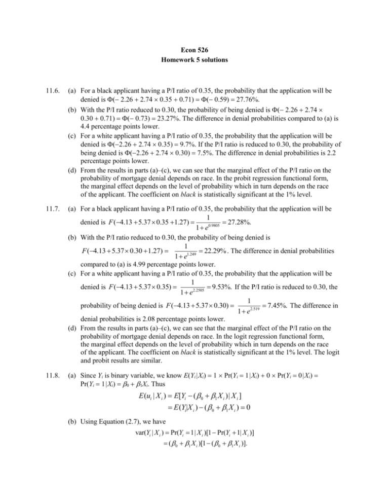
Econ 526
Homework 5 solutions
11.6.
(a) For a black applicant having a P/I ratio of 0.35, the probability that the application will be
denied is ( 2.26  2.74  0.35  0.71)  (0.59)  27.76%.
(b) With the P/I ratio reduced to 0.30, the probability of being denied is ( 2.26  2.74 
0.30  0.71)  (0.73)  23.27%. The difference in denial probabilities compared to (a) is
4.4 percentage points lower.
(c) For a white applicant having a P/I ratio of 0.35, the probability that the application will be
denied is (2.26  2.74  0.35)  9.7%. If the P/I ratio is reduced to 0.30, the probability of
being denied is (2.26  2.74  0.30)  7.5%. The difference in denial probabilities is 2.2
percentage points lower.
(d) From the results in parts (a)–(c), we can see that the marginal effect of the P/I ratio on the
probability of mortgage denial depends on race. In the probit regression functional form,
the marginal effect depends on the level of probability which in turn depends on the race
of the applicant. The coefficient on black is statistically significant at the 1% level.
11.7.
(a) For a black applicant having a P/I ratio of 0.35, the probability that the application will be
1
denied is F (4.13  5.37  0.35 1.27) 
 27.28%.
1  e0.9805
(b) With the P/I ratio reduced to 0.30, the probability of being denied is
1
F (4.13  5.37  0.30  1.27) 
 22.29% . The difference in denial probabilities
1  e1.249
compared to (a) is 4.99 percentage points lower.
(c) For a white applicant having a P/I ratio of 0.35, the probability that the application will be
1
denied is F (4.13  5.37  0.35) 
 9.53%. If the P/I ratio is reduced to 0.30, the
1  e2.2505
1
probability of being denied is F (4.13  5.37  0.30) 
 7.45%. The difference in
1  e2.519
denial probabilities is 2.08 percentage points lower.
(d) From the results in parts (a)–(c), we can see that the marginal effect of the P/I ratio on the
probability of mortgage denial depends on race. In the logit regression functional form,
the marginal effect depends on the level of probability which in turn depends on the race
of the applicant. The coefficient on black is statistically significant at the 1% level. The logit
and probit results are similar.
11.8.
(a) Since Yi is binary variable, we know E(Yi |Xi)  1  Pr(Yi  1|Xi)  0  Pr(Yi  0|Xi) 
Pr(Yi  1|Xi)   0  1Xi. Thus
E (ui | X i )  E[Yi  (  0  1 X i )| X i ]
 E (Yi|X i )  (  0  1 X i )  0
(b) Using Equation (2.7), we have
var(Yi | X i )  Pr(Yi  1| X i )[1  Pr(Yi  1| X i )]
 ( 0  1 X i )[1  (  0  1 X i )].
Thus
var(ui | X i )  var[Yi  (  0  1 X i )i | X i ]
 var(Yi | X i )  ( 0  1 X i )[1  ( 0  1 X i )].
(c) var(ui |Xi) depends on the value of Xi, so ui is heteroskedastic.
 s
 0   0 uid  uis
; thus cov( P, u s )  u

1
1
1
2
12.8.
(a) Solving for P yields P 
(b) Because cov(P,u)  0, the OLS estimator is inconsistent (see (6.1)).
(c) We need a instrumental variable, something that is correlated with P but uncorrelated with us.
In this case Q can serve as the instrument, because demand is completely inelastic (so that Q
is not affected by shifts in supply). 0 can be estimated by OLS (equivalently as the sample
mean of Qi).
12.9.
(a) There are other factors that could affect both the choice to serve in the military and annual
earnings. One example could be education, although this could be included in the regression
as a control variable. Another variable is “ability” which is difficult to measure, and thus
difficult to control for in the regression.
(b) The draft was determined by a national lottery so the choice of serving in the military was
random. Because it was randomly selected, the lottery number is uncorrelated with individual
characteristics that may affect earning and hence the instrument is exogenous. Because it
affected the probability of serving in the military, the lottery number is relevant.