Supporting Information
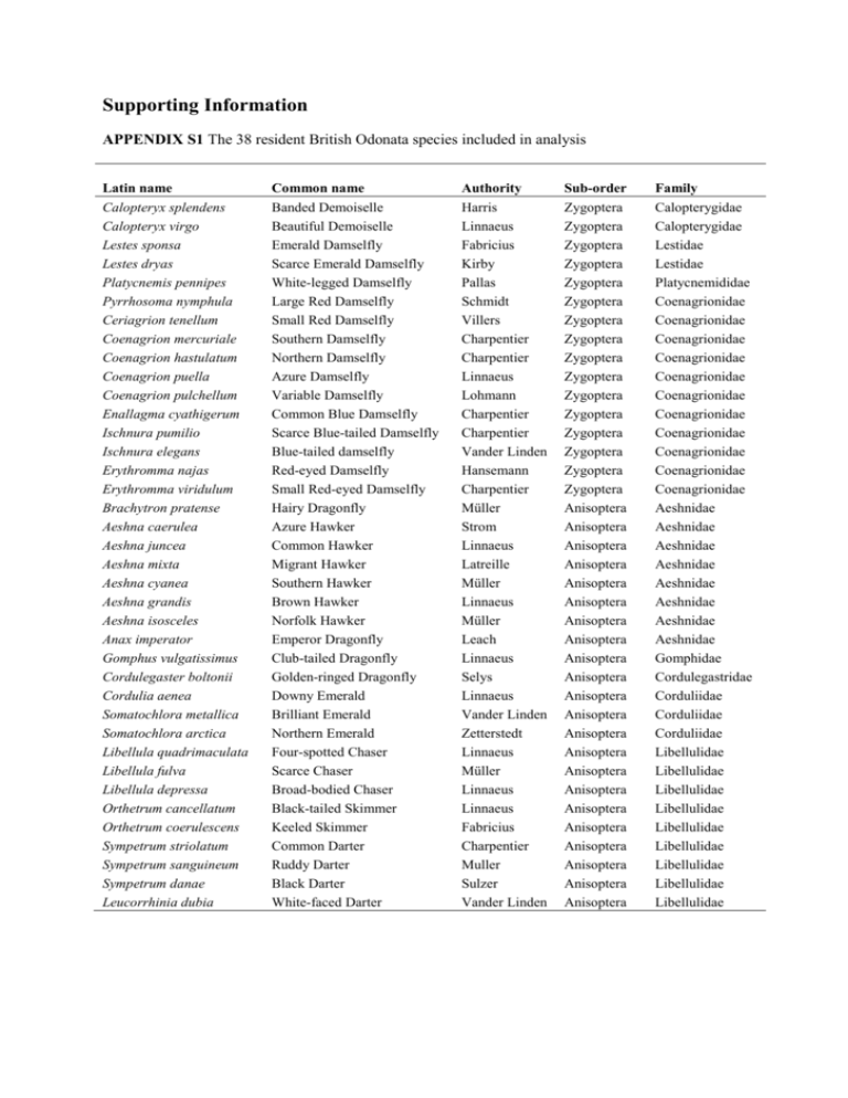
APPENDIX S1 The 38 resident British Odonata species included in analysis
Latin name
Calopteryx splendens
Calopteryx virgo
Lestes sponsa
Lestes dryas
Platycnemis pennipes
Pyrrhosoma nymphula
Ceriagrion tenellum
Coenagrion mercuriale
Coenagrion hastulatum
Coenagrion puella
Coenagrion pulchellum
Enallagma cyathigerum
Ischnura pumilio
Ischnura elegans
Erythromma najas
Erythromma viridulum
Brachytron pratense
Aeshna caerulea
Aeshna juncea
Aeshna mixta
Aeshna cyanea
Aeshna grandis
Aeshna isosceles
Anax imperator
Gomphus vulgatissimus
Cordulegaster boltonii
Cordulia aenea
Somatochlora metallica
Somatochlora arctica
Libellula quadrimaculata
Libellula fulva
Libellula depressa
Orthetrum cancellatum
Orthetrum coerulescens
Sympetrum striolatum
Sympetrum sanguineum
Sympetrum danae
Leucorrhinia dubia
Common name
Banded Demoiselle
Beautiful Demoiselle
Emerald Damselfly
Scarce Emerald Damselfly
White-legged Damselfly
Large Red Damselfly
Small Red Damselfly
Southern Damselfly
Northern Damselfly
Azure Damselfly
Variable Damselfly
Common Blue Damselfly
Scarce Blue-tailed Damselfly
Blue-tailed damselfly
Red-eyed Damselfly
Small Red-eyed Damselfly
Hairy Dragonfly
Azure Hawker
Common Hawker
Migrant Hawker
Southern Hawker
Brown Hawker
Norfolk Hawker
Emperor Dragonfly
Club-tailed Dragonfly
Golden-ringed Dragonfly
Downy Emerald
Brilliant Emerald
Northern Emerald
Four-spotted Chaser
Scarce Chaser
Broad-bodied Chaser
Black-tailed Skimmer
Keeled Skimmer
Common Darter
Ruddy Darter
Black Darter
White-faced Darter
Authority
Harris
Linnaeus
Fabricius
Kirby
Pallas
Schmidt
Villers
Charpentier
Charpentier
Linnaeus
Lohmann
Charpentier
Charpentier
Vander Linden
Hansemann
Charpentier
Müller
Strom
Linnaeus
Latreille
Müller
Linnaeus
Müller
Leach
Linnaeus
Selys
Linnaeus
Vander Linden
Zetterstedt
Linnaeus
Müller
Linnaeus
Linnaeus
Fabricius
Charpentier
Muller
Sulzer
Vander Linden
Sub-order
Zygoptera
Zygoptera
Zygoptera
Zygoptera
Zygoptera
Zygoptera
Zygoptera
Zygoptera
Zygoptera
Zygoptera
Zygoptera
Zygoptera
Zygoptera
Zygoptera
Zygoptera
Zygoptera
Anisoptera
Anisoptera
Anisoptera
Anisoptera
Anisoptera
Anisoptera
Anisoptera
Anisoptera
Anisoptera
Anisoptera
Anisoptera
Anisoptera
Anisoptera
Anisoptera
Anisoptera
Anisoptera
Anisoptera
Anisoptera
Anisoptera
Anisoptera
Anisoptera
Anisoptera
Family
Calopterygidae
Calopterygidae
Lestidae
Lestidae
Platycnemididae
Coenagrionidae
Coenagrionidae
Coenagrionidae
Coenagrionidae
Coenagrionidae
Coenagrionidae
Coenagrionidae
Coenagrionidae
Coenagrionidae
Coenagrionidae
Coenagrionidae
Aeshnidae
Aeshnidae
Aeshnidae
Aeshnidae
Aeshnidae
Aeshnidae
Aeshnidae
Aeshnidae
Gomphidae
Cordulegastridae
Corduliidae
Corduliidae
Corduliidae
Libellulidae
Libellulidae
Libellulidae
Libellulidae
Libellulidae
Libellulidae
Libellulidae
Libellulidae
Libellulidae
APPENDIX S2 Supplementary Methods
a. Threshold species list length for inclusion of cells
There are a number of sources of bias when estimating the occupancy-area relationship (OAR) from
unstructured records of species’ occurrences. It is important to acknowledge that the species recorded
in a cell are not always a complete list of those species present. A single species may have been
recorded because it is particularly charismatic or rare, while a number of more common species
present are not recorded. As such, common species tend to be under-represented, while rare species
are over-represented. One method of addressing this bias is to exclude cells with a species list length
falling below some threshold, hence excluding cells which are likely to be an incomplete list of the
species present. However, this is also problematic as the number of cells available for the analysis
declines steeply as the threshold species list length becomes higher. The list length results in large
losses of cells at fine-grains and very little loss of cells at coarse grains (Fig. S1), therefore proportion
occupancy at the finest spatial grains increases rapidly as the list length threshold gets higher. For
some species this results in a spurious non-monotonic OAR when the list length threshold is high (e.g.
Somatochlora metallica at list length 6, Fig. S2). Moreover, the cells excluded are not spatially
random. In fact, cells that are poorly sampled and those that are less speciose are more likely to be
lost as the threshold species list length is increased. Odonata diversity decreases from South to North
in Britain, as does sampling intensity. Therefore, higher list length thresholds for inclusion of cells
introduce spatial biases into our estimates of distribution size: cells are more likely to be excluded in
the North, so the distribution size will be heavily influenced by the most species-rich and wellsampled regions in the south-east (Fig. S3). The choice of the threshold species list length for
including cells is, therefore, a trade-off between these two sources of bias (under-recording of
common species and spatial bias in estimates of distribution size). Our choice of a list length of >= 1
for inclusion of cells in the analysis reflects this trade-off. In any case, the choice of list length does
not substantially affect the observed OARs for any species in our analysis (Table S1).
Fig. S1 Decline in the number of cells available for analysis as the species list length threshold
increases.
Fig. S2 Effect of species list length threshold on the OAR for 38 British Odonata species. Dark red is the OAR when cells with a species list length of <=0
are included in the analysis. The colour spectrum towards blue represents increasing list length thresholds.
Fig. S3 Spatial patterns of A) species richness and B) sampling intensity in British Odonata records
at the 100km2 grain. Species richness is the number of species recorded in each 100km2 cell between
1990 and 2012. Sampling intensity (# 1km2 cells) is measured as the number of 1km2 cells visited
within each 100km2 cell between 1990 and 2012.
Table S1 Correlations between OARs estimated using a list length of 1 and six other list length
thresholds for the 38 British Odonata species.
List length threshold
Species
0
1
2
3
4
5
6
Aeshna caerulea
0.999901
1
0.999997
0.999972
0.999971
0.999904
0.999888
Aeshna cyanea
0.993162
1
0.998907
0.996996
0.993226
0.987672
0.979178
Aeshna grandis
0.982596
1
0.992985
0.973081
0.919701
0.798752
0.486339
Aeshna isosceles
0.998582
1
0.999777
0.999285
0.998532
0.997285
0.99517
Aeshna juncea
0.999029
1
0.999938
0.999916
0.999937
0.99987
0.999819
Aeshna mixta
0.990633
1
0.998336
0.995696
0.990177
0.981692
0.966379
Anax imperator
0.991143
1
0.997349
0.9899
0.97193
0.935577
0.861896
Brachytron pratense
0.998318
1
0.999754
0.999303
0.998424
0.997019
0.995226
Calopteryx splendens
0.99186
1
0.999436
0.998632
0.997245
0.99469
0.992184
Calopteryx virgo
0.996661
1
0.999799
0.999416
0.998547
0.997343
0.996147
Ceriagrion tenellum
0.999394
1
0.999906
0.999711
0.999366
0.998862
0.998133
Coenagrion hastulatum
0.99994
1
0.999992
0.999979
0.999953
0.999925
0.999914
Coenagrion mercuriale
0.999724
1
0.999965
0.999886
0.999782
0.999643
0.99954
Coenagrion puella
0.989157
1
0.995866
0.985878
0.965299
0.930885
0.871851
Coenagrion pulchellum
0.999804
1
0.999978
0.999944
0.999875
0.999762
0.999667
Cordulegaster boltonii
0.997676
1
0.999941
0.999915
0.999885
0.999869
0.99991
Cordulia aenea
0.999402
1
0.999903
0.999703
0.999359
0.998824
0.998085
Enallagma cyathigerum
0.997772
1
0.999742
0.999729
0.999288
0.998402
0.997047
Erythromma najas
0.996892
1
0.999445
0.998407
0.995899
0.991167
0.983815
Erythromma viridulum
0.999388
1
0.999934
0.999835
0.999605
0.999199
0.99889
0.9987
1
0.999843
0.99959
0.999304
0.999029
0.998785
Ischnura elegans
0.991948
1
0.996968
0.991903
0.985556
0.978561
0.96907
Ischnura pumilio
0.999736
1
0.999968
0.999919
0.999814
0.999656
0.999538
Lestes dryas
0.999667
1
0.999967
0.999907
0.999802
0.999651
0.999527
Lestes sponsa
0.999345
1
0.999954
0.999857
0.999534
0.998907
0.99801
Leucorrhinia dubia
0.999953
1
0.999995
0.999986
0.999977
0.999956
0.999939
Libellula depressa
0.997274
1
0.999492
0.998307
0.995429
0.989021
0.977838
Libellula fulva
0.999266
1
0.999922
0.999786
0.999538
0.999115
0.998809
Libellula quadrimaculata
0.998981
1
0.999923
0.999861
0.999679
0.999218
0.998999
Orthetrum cancellatum
0.997004
1
0.999541
0.998794
0.997107
0.994206
0.990095
Orthetrum coerulescens
0.99931
1
0.999936
0.999832
0.999721
0.999543
0.999488
Platycnemis pennipes
0.996231
1
0.99937
0.998478
0.997396
0.996251
0.995777
Pyrrhosoma nymphula
0.998674
1
0.999712
0.999385
0.998523
0.99724
0.995775
Somatochlora arctica
0.999882
1
0.999988
0.999976
0.999919
0.999886
0.999902
Somatochlora metallica
0.999502
1
0.999918
0.999726
0.999401
0.998885
0.998081
Sympetrum danae
0.999462
1
0.999972
0.999913
0.99977
0.999705
0.999653
Sympetrum sanguineum
0.996054
1
0.999247
0.997869
0.994942
0.989709
0.98292
Sympetrum striolatum
0.991396
1
0.998239
0.996886
0.99492
0.993721
0.992534
Gomphus vulgatissimus
b. Threshold proportion land for inclusion of cells
An additional source of bias is the inclusion of cells with large proportions of sea. Following the
species-area relationship, fewer species will be present in a cell containing a greater proportion of sea.
This introduces a negative bias in distribution size. This can be addressed by excluding cells with the
proportion of land below a specified threshold. However, the number of cells included in the analysis
declines rapidly as the threshold of land required increases, particularly at coarse grains, where large
proportions of cells in the North and South West are sea. When the threshold land is set very high,
the disproportionate loss of coarse grain cells leads to a positive bias in coarse-grain occupancy. Our
choice of 0.3 as the threshold proportion of land required for inclusion of a cell is a trade-off between
the total number of cells in the analysis at each spatial grain and the total amount of land represented
by these cells (Fig. S4).
The threshold proportion of land and the threshold species list length for inclusion of a cell can also
drive different patterns of bias at different spatial grains. In particular, if disproportionately more
cells are excluded at fine grains due to the chosen thresholds, then occupancy at fine grains can be
spuriously higher than at coarser grains, generating a non-monotonic OAR. This is clearly not
possible and cannot be fitted by downscaling models.
Fig. S4 Trade-off between the total proportion land in the study region (dashed black line) and
proportion of cells included in the analysis (solid black line). The vertical dashed lines are the
threshold proportion of land we required to include cells in the analysis (0.3). The same threshold
was used for cells at all spatial grains.
c. Details of downscaling models
The formulae and notation of the ten downscaling models are defined below. The Hui model
(model 1) uses information at single spatial grain, while Models 2 to 9 are fitted to multiple
coarse grains to estimate scale invariant parameters from which the OAR is extrapolated to
finer grains. Consequently, models 2 to 9 are expressed in terms of pA, the proportion of
occupied cells at grain A in a study region of size A0. Following Azaele et al. (2012), the free
parameters of downscaling models 2 to 9 (shown in bold after each formula) were estimated
for each species by numerical minimisation of the Euclidean norm of predicted occupancy in
log space,
1
𝑁
2
𝑝𝑟𝑒𝑑
𝑝𝑟𝑒𝑑
𝑜𝑏
𝑜𝑏
∑𝑔𝐴=1(log 𝑝𝐴,𝑖
− log 𝑝𝐴,𝑖
) , where 𝑝𝐴,𝑖
and 𝑝𝐴,𝑖
are the predicted and
observed occupancy at grain A for species i and g is the number of grains used to
parameterise the model. To estimate the parameters of the Thomas model, a simulated
annealing optimisation algorithm was specified to ensure a robust search for the global
minimum (Bolker, 2008). All optimisation was carried out in Mathematica 9.0 Student
Edition. It should be noted that the Thomas model, like the Hui model, can be used to
downscale with occupancy data at a single spatial grain, provided that information about the
positions of occupied cells is used to parameterise the model.
1) Hui
The Hui model (Hui et al. 2006; Hui 2009) was developed by to describe the spatial scaling
of species occupancy.
The scaling pattern uses conditional probabilities (joint-count
statistics) as well as probability of presence to describe the distribution of a species within a
presence-absence grid. The scaling pattern describes how these probabilities depend on a
percolation process as neighbouring fine-grain cells are combined into larger coarse-grain
cells. Here, we use the model to predict the probability of occupancy at fine grains (the target
grain), using observed occupancy data at a coarser reference grain.
The relationships
between these probabilities can be defined using Bayes’ theorem, such that all conditional
probabilities can be expressed in terms of two pieces of information estimated from spatially
referenced occurrence data at the reference grain: in this case, species atlas data at 10km x
10km (100km2). The first piece of information required is occupancy, the probability that a
randomly chosen cell is occupied; the second, a measure of spatial aggregation, is the
conditional probability that, given a cell is occupied, a randomly chosen cell adjacent to it is
also occupied. The notation for these probabilities and the joint-count statistics are defined
below, along with the relationships between them. We use upper case letters to refer to
observed probabilities at the reference grain and lower case letters to refer to estimated
probabilities at the target (fine) grain.
𝑷+ : observed probability of presence, obtained at the reference grain of the data (100 km2)
𝑸+|+ : observed conditional probability, obtained at the reference grain of the data, that a
randomly chosen cell adjacent to a given occupied cell is also occupied.
𝑷𝟎 : observed probability of absence at the reference grain. P0 = 1 − 𝑃+
𝑸𝟎|𝟎 :, observed conditional probability that a randomly chosen cell adjacent to an empty cell
is also empty. This can be calculated from 𝑄+|+ and 𝑃+ using Bayes’ theorem 𝑄0|0 = 1 −
((1 − 𝑄+|+ ) 𝑃+ ⁄(1 − 𝑃+ )
𝒑+ : estimated probability of presence at the finer, target grain
𝒒+|+ : estimated conditional probability at the finer, target grain that a randomly chosen cell
adjacent to a given occupied cell is also occupied
𝒑𝟎 : estimated probability of absence at the finer, target grain, 1 − 𝑝+
𝒒𝟎|𝟎 : estimated conditional probability, at the finer target grain, that a randomly chosen cell
adjacent to an empty cell is also empty
𝒒𝟎|+ : estimated conditional probability, at the finer target grain, that a randomly chosen cell
adjacent to an occupied cell is empty
𝒒+|𝟎 : estimated conditional probability, at the finer target grain, that a randomly chosen cell
adjacent to an empty cell is occupied
𝒃𝟎 : conditional probability that a cell with two empty neighbours is also empty at the finer,
target grain
n : an index of spatial grain (or the linear grain size). One cell at the reference grain has an
area of n2 cells at the finer, target grain (e.g. to estimate occupancy at 2km x 2km using the
reference grain of 10km x 10km, n = 10/2 = 5). The value of n does not need to be an
integer.
The formula we use to estimate occupancy with the Hui model is derived from equations 6
and 7 in Hui (2009):
2
𝑃0 = 𝑝0 . 𝑞0|0 2(𝑛−1) . 𝑏0 (𝑛−1)
(Eqn. A)
𝑄0|0 = 𝑞0|0 𝑛 . 𝑏0 𝑛(𝑛−1)
(Eqn. B)
The two unknown terms, 𝑞0|0 and 𝑏0 can be expressed in terms of 𝑝0 , 𝑃0 and 𝑄0|0 . This is
achieved for the term 𝑄0|0 by rearranging equations 6 and 7 equal to b0 (and hence to each
other). This equation can then be expressed in terms of the unknown term:
−1
1
1
𝑞0|0 = 𝑝0 −𝑛−1 . 𝑃0 𝑛−1 . 𝑄0|0 𝑛
(Eqn. C)
By substituting equation C into Bayes’ theorem relating the conditional probabilities we can
express the conditional probability 𝑞0|+ in terms of 𝑝0 , 𝑃0 and 𝑄0|0 :
1
𝑞0/+ =
1
−1
−
𝑝0 (1−𝑝0 𝑛−1 𝑃0 𝑛−1 𝑄0|0 𝑛 )
(Eqn. D)
1−𝑝0
We can now express b0 in terms of 𝑝0 , 𝑃0 and 𝑄0|0 , using equation 3 in Hui (2009):
𝑏0 = 𝑞
𝑞0|0 2 .𝑝0
2 .𝑝 + 𝑞
2
0
0|0
0|+ .𝑝+
(Eqn. E)
Equations C and D are substituted into equation D to estimate the unknown 𝑏0 :
2
−2
2
(𝑝0 .1−𝑛−1 . 𝑃0 𝑛−1 . 𝑄0|0 𝑛 )
𝑏0 =
1
(𝑝0
2
1−𝑛−1
. 𝑃0
2
𝑛−1
. 𝑄0|0
−2
𝑛
1
−1
2
𝑝0 2 . (1 − 𝑝0 −𝑛−1 . 𝑃0 𝑛−1 . 𝑄0|0 𝑛 )
+
)
1 − 𝑝0
Finally, the Hui model scaling relationship in Eqn. A can be rewritten, substituting in
𝑞0|0 and 𝑏0 as defined in equations C and E to obtain: 𝑃0 =
(𝑛−1)2
𝑝0 . (𝑝0
1
−𝑛−1
. 𝑃0
1
𝑛−1
(𝑝0
−1 2(𝑛−1)
𝑛
. 𝑄0|0 )
2
2
−2
1−𝑛−1
. 𝑃0 𝑛−1 . 𝑄0|0 𝑛 )
(Eqn. F)
1
1
−1 2
−𝑛−1
2
. 𝑃0 𝑛−1 . 𝑄0|0 𝑛 )
2
2
−2 𝑝0 .(1−𝑝0
1−
𝑝0 𝑛−1 . 𝑃0𝑛−1 . 𝑄0|0 𝑛 +
1−𝑝0
((
))
Note that 𝑝0 in equation F is the only unknown variable. In the absence of an analytical
solution, the value of 𝑝0 is estimated by finding the numerical root of the above equation,
using an iterative algorithm to find successively better approximations to the root. The
predicted value of 𝑝0 is that which satisfies the relationship above for the observed values of
𝑃0 and 𝑄0|0 at the reference grain. Predicted occupancy is then 𝑝+ = 1 - 𝑝0 .
2) Nachman
𝑧
𝑝𝐴 = 1 − 𝑒 −𝑐𝐴
c : constant
z : constant
3) Power Law
𝑝𝐴 = 𝑐𝐴𝑧
c : constant
z : constant
4) Logistic
𝑐𝐴𝑧
𝑝𝐴 =
,
1+ 𝑐𝐴𝑧
c : constant
z : constant
5) Thomas
𝑝𝐴 = 1 − exp {−𝜌 ∫ [1 − exp (−µ ∫𝐴 𝑘(||𝑐⃗ − 𝑥⃗||) 𝑑𝑥⃗)] 𝑑𝑐⃗}
ρ : intensity of the Poisson distribution of cluster centres in a Thomas spatial point process
σ2: variance of the bivariate normal distribution of points around cluster centres
μ : mean number of points around each cluster centre
6) Finite Negative Binomial
𝑝𝐴 = 1 −
𝐴 𝑘
𝐴 𝑘
Г(𝑁+ 0 −𝑘)Г( 0 )
𝐴
𝐴
𝐴 𝑘
𝐴 𝑘
Г (𝑁+ 0 ) Г( 0 − 𝑘)
𝐴
𝐴
N : total number of individuals
A0 : total area of study region
7) Generalised Negative Binomial
𝑐𝐴𝑧 −𝑘
𝑝𝐴 = 1 − (1 +
)
𝑘
c : constant
z : constant
k: overdispersion parameter of a negative binomial distribution
8) Improved negative binomial
𝛾𝐴
𝑝𝐴 = 1 − [𝑐(𝛾𝐴)𝑏−1 ] 1−𝑐(𝛾𝐴)𝑏−1
γ: mean density
b: constant
c: constant
9) Negative Binomial
𝛾𝐴 −𝑘
𝑝𝐴 = 1 − (1 + )
𝑘
γ: mean density
k: overdispersion parameter of the negative binomial distribution
10) Poisson
𝑝𝐴 = 1 − 𝑒 −𝛾𝐴
γ: mean density
d. Species distribution type
In the trait analysis, the predictor distribution type is intended to capture two components of
species’ distributions: the size of the distribution and the spatial arrangement of occupied
cells. Distribution type was initially classified by eye, using distribution maps of British
Odonata at the 100km2 grain. Four discrete categories were identified: Climatic Range Limit
(a large range size with a Northern, Southern, Continental (South Easterly) or Oceanic
(Westerly) distribution), Widespread (a large range size with a distribution throughout British
mainland), Local-aggregated (a small range size, with a largely contiguous distribution), and
Local-sparse (a small range size with a disjunct distribution). In order to confirm that these
categories were borne out in the data, we plotted each species on two axes quantifying the
distribution size (area of occupancy) and spatial arrangement of occupied cells (residuals of
the relationship between occupancy and fractal dimension (Wilson et al., 2004) for grains
100km2 and 10000km2). Seven species changed category (Fig. S5).
Fig. S5 Classification of species’ distribution type for the trait analysis. The colour of circles
indicates the initial classification of distribution type. Blue = widespread, black = climatic range
limit, red = local-aggregated, yellow = local-sparse. The dashed lines denote the revised division of
species into the four categories of distribution type, based on quantifying distribution size and the
spatial arrangement of occupied cells. The labels in the margins define the four categories, L = local
(occupancy < 20 000 km2), RL = range limited (20 000 km2 < occupancy < 125 000 km2), W =
widespread (occupancy > 125 000 km2), Ag = aggregated (residual D > 0 ), Sp = sparse (residual D <
0).
e. Upper quartile of dispersal distances
In the absence of field-based dispersal estimates for many species of British Odonata, dispersal
estimates were taken from R Fitt.
Dispersal distances were inferred from the distances of newly
colonised 1km2 cells in each year from the nearest previously occupied cell. The 75th percentile of all
dispersal distances between 1991 and 2012 was used as the measure of species-level dispersal in the
trait analysis (75% of newly colonised cells for the focal species were within this distance of the
nearest occupied cell). False absences can lead to overestimates of dispersal from distribution data
when high percentiles from the dispersal kernel are used to infer dispersal.
However, lower
percentiles conceal much of the interspecific variation in dispersal, because most individuals of any
species will disperse very short distances, while only a few individuals will disperse far. Our use of
the 75th percentile of the dispersal kernal reflects this trade-off between the stronger signal (more
interspecific variation) and greater noise (less certainty in the estimates of dispersal) at the highest
percentiles of the dispersal kernel (see Fig. S6).
Fig. S6 Effect of species’ dispersal on the percentage error of downscaling predictions using different
quantiles of the dispersal kernel as the estimate of dispersal distance. Red circles are Zygoptera
(damselflies) and black circles are Anisoptera (dragonflies), indicating there is no clear phylogenetic
signal in dispersal distance, despite the body size differences between dragonflies and damselflies.
f. Odonata Phylogeny
To control for phylogenetic non-independence among the traits of related taxa, we attempted to build
a phylogeny based on genetic distances for all 38 British Odonata species in the analysis. Due to a
lack of suitable genetic data for a large number of Odonata species and low confidence in alignments,
we instead used a phylogeny based on species taxonomy. We converted the taxonomy (Suborder,
Family, Genus, Species) into a tree with polytomies at each node and branch lengths set to 1 using the
as.phylo function from the R package ape (Paradis et al., 2004).
APPENDIX S3 Supplementary Results
a. Comparison of downscaling models for British Odonata.
Model performance was assessed using the absolute values of percentage errors and the raw
percentage errors of downscaling predictions for 114 species:grain combinations are shown in Table
S2. Absolute values of percentage errors are a better measure of overall predictive accuracy, as they
avoid averaging across positive and negative errors with a model and cancelling out predictive error.
However, raw percentage errors are also useful as they provide information about positive or negative
bias in downscaling predictions.
Table S2 Summary of percentage errors and absolute percentage errors of downscaling predictions. Median, min and max are the absolute percentage error of downscaling
predictions at three spatial grains. Best is the number of species for which each model gave the best predictions (the lowest mean percentage error for each species).
% errors
2
Spatial Grain (km )
Model
25
4
1
Median
Min
Max
Best
Median
Min
Max
Best
Median
Min
Max
Best
2.946
-29.347
24.097
12
22.548
-34.342
64.685
12
32.737
-39.094
102.467
15
Nachman
-0.299
-35.276
35.974
8
-13.044
-67.252
49.709
9
-36.33
-85.121
66.136
10
Power Law
10.716
-34.304
43.698
4
16.924
-66.161
105.869
7
14.429
-83.639
126.543
5
Logistic
-8.188
-36.218
30.889
5
-40.254
-77.808
36.904
5
-62.254
-93.259
42.914
4
Thomas
-27.166
-75.158
44.877
2
-72.386
-94.513
74.985
1
-90.219
-98.518
28.74
3
Finite Negative Binomial
-35.67
-60.819
5.274
1
-78.67
-91.12
-0.835
2
-92.945
-97.591
-34.52
1
Generalised Negative Binomial
-7.142
-57.789
14.412
3
-34.711
-93.37
2.101
0
-58.524
-99.515
-2.521
0
Improved Negative Binomial
-9.629
-38.587
10.817
2
-37.629
-72.525
1.561
2
-62.436
-89.026
-3.476
0
Negative Binomial
-30.189
-64.27
4.584
1
-74.42
-92.094
-3.166
0
-90.989
-97.863
-37.531
0
Poisson
-67.962
-84.497
-46.648
0
-91.111
-96.759
-82.29
0
-97.181
-99.132
-93.859
0
Hui
Absolute value of % errors
2
Spatial Grain (km )
Model
25
4
1
Median
Min
Max
Best
Median
Min
Max
Best
Median
Min
Max
Best
Hui
5.566
0.313
29.347
12
24.314
1.663
64.685
12
36.231
0.739
102.467
15
Nachman
7.562
0.234
35.974
8
23.371
0.197
67.252
9
41.090
0.119
85.121
10
Power Law
14.632
0.434
43.698
4
29.901
0.202
105.869
7
42.649
2.930
126.543
5
Logistic
14.501
0.548
36.218
5
40.254
2.053
77.808
5
62.254
6.367
93.259
4
Thomas
28.164
0.457
75.158
2
73.663
6.213
94.513
1
90.219
2.254
98.518
3
Finite Negative Binomial
35.670
2.191
60.819
1
78.670
0.835
91.120
2
92.945
34.520
97.591
1
7.416
0.240
57.789
3
34.711
0.209
93.370
0
58.524
2.521
99.515
0
Improved Negative Binomial
10.725
0.363
38.587
2
37.629
0.080
72.525
2
62.436
3.476
89.026
0
Negative Binomial
30.189
0.473
64.270
1
74.420
3.166
92.094
0
90.989
37.531
97.863
0
Poisson
67.962
46.648
84.497
0
91.111
82.290
96.759
0
97.181
93.859
99.132
0
Generalised Negative Binomial
b. Trait analysis
Table S3 Unstandardised parameter estimates for the trait analysis. We tested for an effect of four
species-level traits on the predictive error of the Hui downscaling model using a linear model. The
global model was Percentage Error ~ Distribution type + log10 Dispersal ability + Range change+
Habitat breadth. Weighted model averaging was used to obtain parameter estimates for each trait
with the lower and upper 95% confidence intervals. Parameter estimates are averaged across three
models with ΔAIC < 4, weighted by the Akaike weights of each model. The reference group of the
factor distribution type is Climatic Range Limit. The trait variables are ordered by decreasing relative
importance.
Parameter
Estimate
Lower 95% CI
Upper 95% CI
0.725
-21.341
35.851
Distribution type local-aggregated
-35.626
-63.257
-7.995
Distribution type local-sparse
-52.763
-73.807
-31.719
Distribution type widespread
-36.795
-58.572
-15.017
Log10 Dispersal ability (km)
89.792
0.222
0.752
Range change (1970-2012)
68.007
-146.781
282.794
Habitat breadth
-0.042
-7.925
7.842
Intercept
Table S4 Generalised variance inflation factors (GVIF) for each of the predictor variables included in
the global model of predictive downscaling error. GVIFs were obtained using the function vif in R
package car (Fox & Weisberg, 2011). All GVIF values are < 4 indicating collinearity does not
severely inflate the variance associated with parameter estimates.
Predictor
Distribution type
log10 Dispersal distance (km)
Range change (1970-2012)
No. habitat types
Generalised
variance
inflation factor
(GVIF)
2.276139
1.203343
1.312466
1.790005
Df
3
1
1
1
GVIF (1/(2*Df))
1.14692
1.09697
1.145629
1.33791
Table S5 Correlation matrix between pairs of traits included the global linear model of predictive
downscaling error.
Predictor
Distribution type
log10 Dispersal distance (km)
Range change
No. habitat types
Distribution
type
1
0.28265
0.39481
0.655771
log10
Dispersal
No. habitat
distance (km) Range change types
0.28265
0.39481
0.655771
1
0.122213
-0.18865
0.122213
1
0.179419
-0.18865
0.179419
1
References
Azaele, S., Cornell, S.J. & Kunin, W.E. (2012). Downscaling species occupancy from coarse
spatial scales. Ecological Applications, 22, 1004–1014.
Bolker, B.M. (2008). Ecological Models and Data in R. Princeton University Press, Oxford.
Fox J. & Weisberg S (2011) An R Companion to Applied Regression. Sage Publications,
Thousand Oaks, CA, USA
Hui, C. (2009). On the scaling patterns of species spatial distribution and association. Journal
of Theoretical Biology, 261, 481–7.
Hui, C., McGeoch, M.A., Reyers, B., le Roux, P.C., Greve, M. & Chown, S.L. (2009).
Extrapolating population size from the occupancy-abundance relationship and the
scaling pattern of occupancy. Ecological Applications, 19, 2038–48.
Hui, C., McGeoch, M.A. & Warren, M. (2006). A spatially explicit approach to estimating
species occupancy and spatial correlation. Journal of Animal Ecology, 75, 140–147.
Paradis E., Claude J. & Strimmer K. (2004) Analyses of phylogenetics and evolution in R
language. Bioinformatics, 20, 289-290
Wilson, R.J., Thomas, C.D., Fox, R., Roy, D.B. & Kunin, W.E. (2004). Spatial patterns in
species distributions reveal biodiversity change. Nature, 432, 393–396.