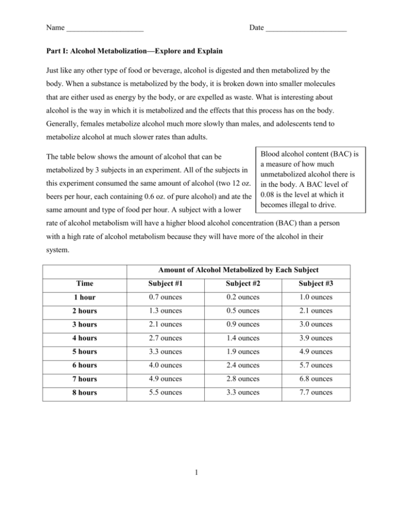
Name ____________________
Date _____________________
Part I: Alcohol Metabolization—Explore and Explain
Just like any other type of food or beverage, alcohol is digested and then metabolized by the
body. When a substance is metabolized by the body, it is broken down into smaller molecules
that are either used as energy by the body, or are expelled as waste. What is interesting about
alcohol is the way in which it is metabolized and the effects that this process has on the body.
Generally, females metabolize alcohol much more slowly than males, and adolescents tend to
metabolize alcohol at much slower rates than adults.
The table below shows the amount of alcohol that can be
metabolized by 3 subjects in an experiment. All of the subjects in
this experiment consumed the same amount of alcohol (two 12 oz.
beers per hour, each containing 0.6 oz. of pure alcohol) and ate the
same amount and type of food per hour. A subject with a lower
Blood alcohol content (BAC) is
a measure of how much
unmetabolized alcohol there is
in the body. A BAC level of
0.08 is the level at which it
becomes illegal to drive.
rate of alcohol metabolism will have a higher blood alcohol concentration (BAC) than a person
with a high rate of alcohol metabolism because they will have more of the alcohol in their
system.
Amount of Alcohol Metabolized by Each Subject
Time
Subject #1
Subject #2
Subject #3
1 hour
0.7 ounces
0.2 ounces
1.0 ounces
2 hours
1.3 ounces
0.5 ounces
2.1 ounces
3 hours
2.1 ounces
0.9 ounces
3.0 ounces
4 hours
2.7 ounces
1.4 ounces
3.9 ounces
5 hours
3.3 ounces
1.9 ounces
4.9 ounces
6 hours
4.0 ounces
2.4 ounces
5.7 ounces
7 hours
4.9 ounces
2.8 ounces
6.8 ounces
8 hours
5.5 ounces
3.3 ounces
7.7 ounces
1
1. Graph the rate of metabolism for each person in the graphs provided below. Make sure to
include all parts of a graph (title, axes titles, etc.), as well as a trend line for each graph.
Amount of Alcohol Metabolized
Metabolization of Subject 1
6
y = 0.6893x - 0.0393
R² = 0.9978
5
4
3
Series1
2
Linear (Series1)
1
0
0
2
4
6
8
10
Time (hours)
Amount of Alcohol Metabolized
Metabolization of Subject 2
3.5
y = 0.4548x - 0.3714
R² = 0.9967
3
2.5
2
Series1
1.5
Linear (Series1)
1
0.5
0
0
2
4
6
8
Time (hours)
2
10
Amount of Alcohol Metabolized
Metabolization of Subject 3
9
y = 0.9464x + 0.1286
R² = 0.9993
8
7
6
5
4
Series1
3
Linear (Series1)
2
1
0
0
2
4
6
8
10
Time (hours)
2. Calculate the average rate of alcohol metabolism for each subject. (Show your work!)
a. Subject 1: 0.689 oz/hour
b. Subject 2: 0.454 oz/hour
c. Subject 3: 0.946 oz/hour
d. How did you calculate the average rate of metabolism? Explain why you chose
this process. There may be a variety of different ways that a student answers these
questions. They may get this answer from the slope of the linear regression, which
is the most accurate way to calculate the rate of metabolism. OR, they may also
take two of the points on the graph and try and calculate slope that way. It is up to
you to determine which answer you consider “correct.”
e. The researcher who gathered this data calculated the average rate of metabolism
two different ways. First the scientist calculated the slope of the linear regression.
Then the scientist took the difference between each hour 8 and hour 1 and then
divided it by 8 (for 8 hours). Which method do you think is more accurate and
why? It is more accurate to calculate the rate of metabolism from the slope
because it takes into account all of the points on the graph and it also accounts for
any outliers in the data.
3
3. Hypothesize the age and gender of subjects 2 and 3. Explain your reasoning.
a. Subject 2: young female, maybe adolescent age (16-20) based on the low rate of
metabolism. Females metabolize alcohol much more slowly than males as do
people who have not been previously exposed to alcohol, so it is assumed that this
person has not really been exposed to alcohol. Answers may vary for this section.
b. Subject 3: older male, maybe 30s or 40s based on the high rate of metabolism.
Males metabolize alcohol much more quickly than females and it is assumed this
person is older because he can metabolize alcohol quickly so he most likely has
been exposed to alcohol for quite some time and a has a tolerance built up.
Answers may vary for this section. This question is here in order to allow students
to begin thinking about how alcohol may affect his/her body.
Part II: Experiment
A researcher wanted to know if there was a difference in the way that the consumption of
alcohol affected adults and adolescents. This researcher designed an experiment that
tested the alcohol metabolism of 8 different people as an adolescent—age 18—and as an
adult—age 30. The experimental setup was the same when the participants were an
adolescent and when they were an adult. Each participant drank two 12 oz. beers every
hour for 8 hours and ate the same type and amount of food throughout the experiment.
The average metabolism of each person per hour is
listed in the table below.
Before becoming a subject in this experiment, each
participant was screened to see if they had the
correct qualifications to be a part of this
experiment. Therefore, each subject has a family
history of alcoholism in their immediate family
going back at least 3 generations (for example,
Alcoholism is an addiction to the
consumption of alcoholic
beverages in which a person is
physically dependent on the
alcohol. If an alcoholic stops
consuming alcohol he/she will
likely have withdrawal effects
because the body is so used to
having alcohol in the system.
father, father’s mother, and father’s grandfather).
Also, none of the subjects showed signs of alcoholism nor did they become alcoholics
before the experiment was concluded. The table below shows the average body weight
and metabolic rate of each subject as an adolescent and as an adult.
4
Body Weight
Adolescent
Body weight as
Adult
as Adolescent
Metabolic Rate
Adult
Metabolic Rate
1
40 kg
0.257 oz/hr
55 kg
0.689 oz/hr
2
48 kg
0.598 oz/hr
59 kg
1.143 oz/hr
3
52 kg
0.454 oz/hr
53 kg
1.022 oz/hr
4
70 kg
0.491 oz/hr
72 kg
0.984 oz/hr
5
61 kg
0.643 oz/hr
67 kg
1.123 oz/hr
6
50 kg
0.342 oz/hr
56 kg
0.887 oz/hr
7
56 kg
0.232 oz/hr
60 kg
0.769 oz/hr
8
75 kg
0.334 oz/hr
75 kg
0.735 oz/hr
Subject #
Note: 100 pounds is equivalent to 45 kg, and 200 pounds is equivalent to 91 kg.
Answer questions 1-5 based on the table above.
1. Why is it important that each person had a family history of alcohol use, but did not
develop alcoholism? It is assumed that if a person has a family history of alcoholism,
he/she will be able to break down more alcohol, and we want this factor to be equal
across all participants.
2. Each of the participants drank 24 oz. of alcohol over the course of 8 hours. Calculate the
grams of alcohol that each participant drank over 8 hours. (Hint: 1 oz. = 28.35 g)
24oz. x 28.35 g/oz.= 680.4 g
Grams Alcohol Consumed: 680.4 g
5
3. Based on the body weight of each subject (as an adult and adolescent), calculate the
grams of alcohol consumed/kilogram of body weight for each subject at both age points.
Display your data in the table provided below.
Subject #
Adolescent (g/kg)
Adult (g/kg)
1
17.01
12.37
2
14.18
11.53
3
13.08
12.84
4
9.72
9.45
5
11.15
10.16
6
13.61
12.15
7
12.15
11.34
8
9.07
9.07
a. What is the purpose of calculating the g alcohol consumed/kg body weight for
each individual if you already know how many ounces of alcohol they consumed?
Because it takes more alcohol for a person with more body mass to feel the effects
of alcohol. Therefore, in order to be able to compare the amount of alcohol drank
across all subjects, it is necessary to convert to g/kg
4. Hypothesize whether or not you think that the metabolic rates of the adults are
significantly higher than the metabolic rates of the adolescents.
Answers will vary for this section.
5. Perform a t-test to determine if the metabolic rates of the adults are significantly higher
than the metabolic rates of the adolescents. Set α = 0.05
Null Hypothesis H˳ = no statistical difference
Specified mean of differences μ˳ = 0
H1 = Adult metabolic rate is higher
Actual Mean of Difference μD = 0.500
Standard deviation of differences: 0.0597
6
Number of Samples: 8
How to Calculate Actual Mean of Difference μD
0.689 – 0.257 = 0.432
Differences added up = 4.001
1.143 – 0.598 = 0.545
1.022 – 0.454 = 0.568
0.984 – 0.491 = 0.493
4.001/8 = 0.500
1.123 – 0.643 = 0.480
0.887 – 0.342 = 0.545
0.769 – 0.232 = 0.537
0.735 – 0.334 = 0.401
How to calculate Standard Deviation of the Differences
1
 (  D  x) 2
n 1
1
(0.5  0.432) 2  (0.5  0.545) 2  (0.5  0.568) 2 ..........(0.5 - 0.401) 2
8 1
 0.0597
How to calculate the t-value
t
 D  
standard deviation of difference
n
0.5  0
t
 23.7
0.0597
8
How to calculate the p-value
Look at the p-value chart that was provided on the website with this lesson plan
t-value: 23.7
p-value<0.001
7
a. Are the results significant? Explain. Make sure to include the size of the sample
and the family histories of the individuals to further expand on your answer.
Yes the results are significant. There is greater than a 99.999% chance that these
results are not due to chance (less than 0.001% that they are due to chance). The
sample size, however, was relatively small, so it is always a good idea to do
further testing in order to prove your hypothesis. All of these individuals had a
family history of alcohol use, which could have caused them to have a genetic
influence that allowed them to metabolize alcohol more quickly. Further testing
should be done to compare people with family history of alcoholism and those
without a family history of alcoholism.
b. You may notice that the t-value that you get for this test is not even on the chart of
t-values. Explain what this means in terms of how significant your results are.
It means that the results are extremely significant, and that you, as a scientist, can
be sure that the results are this specific experiment are not due to chance.
c. Explain why a t-test was more appropriate to use than a chi-square test.
This data was paired—meaning that the metabolic rate of the adult was dependent
on the metabolic rate of the adolescent. In order to compare data that is paired, it
is necessary to look at the differences between the data in order to compare them.
With a chi-square test, you must have a set of data that you expect to gather from
your experiment. So in this case, a paired t-test was more appropriate to use.
8
You may be interested to know that after each hour of alcohol consumption, each subject was
asked to complete a series of physical and mental tests. The physical tests included walking in a
straight line, jumping on one foot without falling down, and balancing on one foot. The mental
tests included recognizing patterns, performing mental math, and reading simple sentences. The
data from hour 0 (before the experiment began), hour 2, and hour 8 are shown in the tables
below. A score of 100 means that the subject completed all tests with no errors, and a score of 0
means that the subject failed every question and every test given.
Hour 0
Subject #
Score as an Adolescent
Score as an Adult
1
84
84
2
95
93
3
90
90
4
91
90
5
97
98
6
84
87
7
85
84
8
89
88
Subject #
Score as an Adolescent
Score as an Adult
1
83
84
2
92
90
3
90
90
4
91
90
5
99
98
6
86
87
7
85
86
8
89
88
Hour 2
9
Hour 8
Subject #
Score as an Adolescent
Score as an Adult
1
76
42
2
86
56
3
86
41
4
83
60
5
92
39
6
80
54
7
81
56
8
84
49
6. Perform a t-test for each of the hours (0, 2, and 8) to determine whether or not the
adolescents have higher scores than the adults. Set your α=0.05. This data was calculated
in the same way as in question #5 above.
a. Hour 0
H˳ = no statistical difference H1 = the adolescents have higher scores
μ˳ = 0
t = 0.227
μD = 0.125
p > 0.5
How to Calculate Actual Mean of Difference μD
84 - 84 = 0
85 – 84 = 1
95 – 93 = 2
89 – 88 = 1
90 – 90 = 0
91 – 90 = 1
Differences added up = 1
97 – 98 = -1
Mean = 1/8 = 0.125
84 – 87 = -3
10
How to calculate Standard Deviation of the Differences
1
(  D  x) 2

n 1
1
(0.125  0) 2  (0.125  2) 2  (0.125  0) 2 ..........(0.125 - 1) 2
8 1
 1.55
How to calculate the t-value
t
 D  
standard deviation of difference
n
0.125  0
t
 0.227
1.55
8
If you look on the chart of critical t-values, a t-value of 0.227 corresponds to a p value
greater than 0.5, which means that there is greater than a 50% chance that the differences
between these data are due to chance.
b. Hour 2
H˳ = no statistical difference H1 = the adolescents have higher scores
μ˳ = 0
t = 0.6070
μD = 0.25
p = 0.5630
How to Calculate Actual Mean of Difference μD
83 – 84 = -1
92 – 90 = 2
90 – 90 = 0
91 – 90 = 1
Differences added up = 2
99 – 98 = 1
86 – 87 = -1
85 – 86 = -1
Mean of Difference = 2/8 = 0.25
89 – 88 = 1
11
How to calculate Standard Deviation of the Differences
1
(  D  x) 2

n 1
1
(0.25  (1)) 2  (0.25  2) 2  (0.25  0) 2 ..........(0.25 - 1) 2
8 1
 1.16
How to calculate the t-value
t
 D  
standard deviation of difference
n
t
0.25  0
 0.607
1.16
8
If you look on the chart of critical t-values, a t-value of 0.607 corresponds to a p value
greater than 0.5, which means that there is greater than a 50% chance that the differences
between these data are due to chance.
c. Hour 8
H˳ = no statistical difference H1 = the adolescents have higher scores
μ˳ = 0
t = 9.17
μD = 33.88
p < 0.005
How to Calculate Actual Mean of Difference μD
76 – 42 = 34
86 – 56 = 30
86 – 41 = 45
83 – 60 = 23
Differences added up = 271
92 – 39 = 53
80 – 54 = 26
81 – 56 = 25
Mean of Difference = 271/8 = 33.88
84 – 49 = 35
12
How to calculate Standard Deviation of the Differences
1
(  D  x) 2

n 1
1
(33.88  34) 2  (33.88  30) 2  (33.88  45) 2 ..........(33.88 - 35) 2
8 1
 10.45
How to calculate the t-value
t
 D  
standard deviation of difference
n
33.88  0
t
 9.17
10.45
8
If you look on the chart of critical t-values, a t-value of 9.17 corresponds to a p value less
than 0.005, which means that there is less than a 95.5% chance that the differences
between these data are due to chance.
d. Based on the results of your t-tests, who performed better on the tests at each time
point?
i. Hour 0: Neither one performed better, the null hypothesis was supported
ii. Hour 2: Neither one performed better, the null hypothesis was supported
iii. Hour 8: The adolescents performed significantly better than the adults
7. Based on these results, why do you think drinking as an adolescent is dangerous?
Answers will vary. You may see some things such as: adolescents cannot metabolize
alcohol very quickly so they get drunk more quickly, adolescents also do not feel the
effects of alcohol as much as adults, so they may continue to drink even though they are
highly intoxicated which can cause a person to get sick (ex. Alcohol poisoning), etc.
13
8. After seeing this data, give an explanation as to why you think that the drinking age was
changed from 18 to 21. Do you agree with the decision to change the drinking age?
It is dangerous for an adolescent to be drinking alcohol for the reasons listed above, so
they changed the drinking age so that adolescents would not have access to alcohol.
Answers will vary for the second part of the question. If you do not want for your
students to debate this topic in your classroom, you are more than welcome to edit out
this question.
14