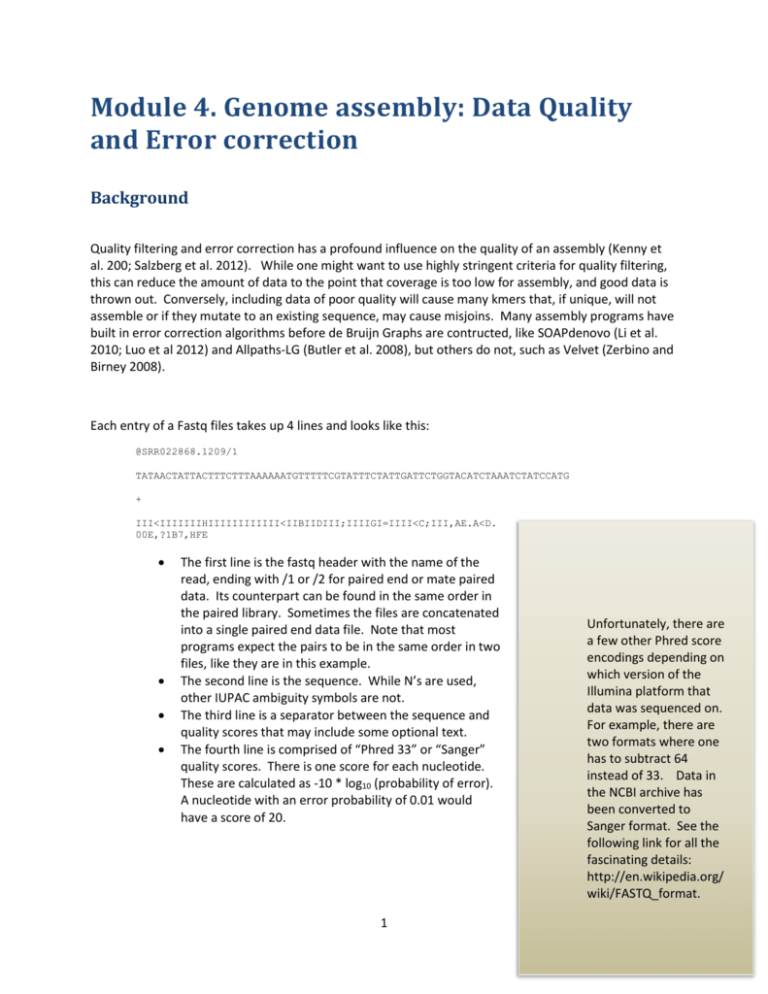
Module 4. Genome assembly: Data Quality
and Error correction
Background
Quality filtering and error correction has a profound influence on the quality of an assembly (Kenny et
al. 200; Salzberg et al. 2012). While one might want to use highly stringent criteria for quality filtering,
this can reduce the amount of data to the point that coverage is too low for assembly, and good data is
thrown out. Conversely, including data of poor quality will cause many kmers that, if unique, will not
assemble or if they mutate to an existing sequence, may cause misjoins. Many assembly programs have
built in error correction algorithms before de Bruijn Graphs are contructed, like SOAPdenovo (Li et al.
2010; Luo et al 2012) and Allpaths-LG (Butler et al. 2008), but others do not, such as Velvet (Zerbino and
Birney 2008).
Each entry of a Fastq files takes up 4 lines and looks like this:
@SRR022868.1209/1
TATAACTATTACTTTCTTTAAAAAATGTTTTTCGTATTTCTATTGATTCTGGTACATCTAAATCTATCCATG
+
III<IIIIIIIHIIIIIIIIIIII<IIBIIDIII;IIIIGI=IIII<C;III,AE.A<D.
00E,?1B7,HFE




The first line is the fastq header with the name of the
read, ending with /1 or /2 for paired end or mate paired
data. Its counterpart can be found in the same order in
the paired library. Sometimes the files are concatenated
into a single paired end data file. Note that most
programs expect the pairs to be in the same order in two
files, like they are in this example.
The second line is the sequence. While N’s are used,
other IUPAC ambiguity symbols are not.
The third line is a separator between the sequence and
quality scores that may include some optional text.
The fourth line is comprised of “Phred 33” or “Sanger”
quality scores. There is one score for each nucleotide.
These are calculated as -10 * log10 (probability of error).
A nucleotide with an error probability of 0.01 would
have a score of 20.
1
Unfortunately, there are
a few other Phred score
encodings depending on
which version of the
Illumina platform that
data was sequenced on.
For example, there are
two formats where one
has to subtract 64
instead of 33. Data in
the NCBI archive has
been converted to
Sanger format. See the
following link for all the
fascinating details:
http://en.wikipedia.org/
wiki/FASTQ_format.
In order for the quality scores to take only one character of space, they are encoded as ASCII
text, each character of which has a numerical, as well as text value. You can find a table with
the values at http://en.wikipedia.org/wiki/ASCII. Note that the integer 33 is represented by “!”
and 73 by “I”. To convert to numerical error probabilities, one would take the decimal value of
the ASCII character (e.g. 73), subtract 33 (73-33=40), divide by -10 (40/-10=-4), and raise 10 to
that value (e.g. 10^-4= 0.0001).
The following boxplot shows Phred quality scores (see above) on the y-axis and position within reads
starting from the 5’ end (for all read simultaneously). Boxplots summarize quality data across the entire
data set for each position. A decline in quality is shown from 5’ to 3’ position. The center of the box is
the median, lower end of the box is the 25th percentile (Q1), top of the box the 75th percentile (Q3),
whiskers show the data at about two standard deviations from the median [>1.5x(Q3-Q1) distant from
Q1 or Q3] and blue stars are outliers.
Reflection Question: Does this look like a good run?
Do you think one could assemble a genome with data of this quality?
Several programs correct errors in reads using kmer graphs in whole genome sequencing projects. To
use the graphs they identify error reads as those below the minimum point between the true and error
kmer peaks. Each putative error kmer is examined for poor quality nucleotides and replacements are
selected based on how their probability, as well as the common errors made by the sequencing
platform.
In order to better separate peaks representing error and true kmers, rather than count each kmer one
time for it’s occurrence the program Quake weights the kmer count by the product of [1-P(error)] over
all nucleotides in the kmer. If all nucleotides in a kmer have very low error probabilities, the qmer count
will be close to the number of kmers. For example, if 15 nucleotides in a kmer all had error probabilities
of 0.01, the qmer count for that kmer would be 0.99^15 = 0.86. On the other hand, a kmer with poor
quality (e.g. p(error) = 0.2 for each of 15 nucleotides) would result in a qmer count much less than one.
2
For example 0.8^15=0.035. Five such kmers would still have a count of less than one (0.035*5=0.18).
Overall, conversion to qmer counts helps to separate true low coverage kmers from error kmers. Quake
will filter out reads that cannot be corrected and still produce low qmers, and will trim poor quality
nucleotides off read ends as well. This step is relatively computationally intensive. We we will use the
HHMI cluster to do this job. In the example below we will see the effects of such error correction on
files containing the S. aureus genome.
Goals




Understand Phred quality scores and construct box plots
Understand how kmer graphs can be used to identify errors in reads
File transfer from HHMI cluster to another cluster (Galaxy)
Optional: Use Galaxy platform
V&C core competencies addressed
1) Ability to apply the process of science: Evaluation of experimental evidence
2) Ability to use quantitative reasoning: Developing and interpreting graphs, Applying statistical
methods to diverse data, Mathematical modeling, Managing and analyzing large data sets
3) Use modeling and simulation to understand complex biological systems:
Applying informatics tools, Managing and analyzing large data sets, Incorporating stochasticity into
biological models
GCAT-SEEK sequencing requirements
Any
Computer/program requirements for data analysis
Linux OS, Quake
Optional Cluster: Qsub
If starting from Window OS: Putty
If starting from Mac OS: SSH
Protocols
A. Log onto the cluster.
B. Make a directory entitled “quake” and enter it.
3
$mkdir quake
$cd quake
C. Move your four raw fastq files for S. aureus from the the jellyfish directory into the working
directory. We could have copied them but proliferating files takes up lots of space.
$mv ~username/jellyfish/*1.fastq .
$mv ~username/jellyfish/*2.fastq .
D. Make a new file and name it at the same time:
$nano fastqfiles
E. List the file names as below. Note that paired reads need to be on the same line of this file.
Once you’ve typed the information below hit control-X and you will be prompted for save
information.
________________________________________________________
frag_1.fastq frag_2.fastq
shortjump_1.fastq shortjump_2.fastq
________________________________________________________
Another Qsub Example
We will be using Qsub to submit our Quake job to the cluster queue. Edit the file ExampleQsubScript to
run quake.py on the cluster like before, using 16 processors on 1 node. See if you can get it to work on
your own by referring to the example in module 2. The command line below comprises the last line of
ExampleQsubScript. Before you run Qsub, check your edits against the file at the end of this module.
quake.py –f fastqfiles –p 16 –k 15
The last line of the file will run quake.py script on 16 (-p 16) processors for a kmer of 15 (-k 15) on all
four data sets at once, maintaining order of paired reads.
Send the job to the worker nodes by entering:
$qsub -p [an integer between -1024 and 1023 with higher values as
priority] [name of script]
e.g. $qsub –p 100 ExampleQsubScript
4
It still may take 10 minutes.
To shows full listing of processes running in Qsub:
$qstat -all
To delete your job if you make a mistake:
$qdel [jobid]
F. Corrected data is in the fastq files with “cor” in the name. 1 bp takes up one Byte of storage
space, so excluding headers, the size in MB = size in BP. Compare the size of the corrected and
uncorrected datasets using:
$ls –la
Optional: Examine quality statistics using Galaxy
a. Go to Galaxy. https://main.g2.bx.psu.edu. Under tools/ get data/upload files from your
computer, in the white space for a URL upload copy/paste:
https://main.g2.bx.psu.edu/datasets/bbd44e69cb8906b5016849ed21004d1f
b. Go to the menu NGS Toolbox QC and Manipulation/Illumina Data/Fastq groomer and select the
file. It is the frag_1.fastq file. The groomer will let Galaxy know the quality scores are in Sanger
format, by hitting execute and making sure the file format is Sanger.
c. Use FASTQ Summary Statistics to summarize fastq scores on the dataset.
d. Use Graphs_DisplayData/Boxplot to make a boxplot of the quality scores.
e. Repeat on the Quake Corrected dataset. You will first need to transfer the file from the cluster
to galaxy.
FTP directly from Cluster to Galaxy
Log onto the cluster using PuTTY, and move into your Quake directory
Launch ftp by:
$ftp
Then open the remote site by:
>open main.g2.bx.psu.edu
You will be prompted for your user name (e-mail address) and password. Enter them.
You are connected to the Penn State servers. To do the transfer
>put frag_1.cor.fastq
To exit out of ftp:
>close
5
f. Go to upload files in Galaxy, and your data should appear with a check box available.
Q. How many reads were filtered out by Quake? Select the file name on the right to expand and read
the file descriptions.
Assessment
Draw boxplots for poor, intermediate and excellent quality data (100bp reads). Label axes.
Examine the qmer histogram file. Compare the peak in the qmer plot to the kmer peak for the same
data in Jellyfish. What does it say about the data for the qmer peak to be shifted and lower?
Draw a qmer plot and label error peaks, true peaks, repeats.
What is the qmer score of 10 nucleotides with a phred score of 10 each.
Redo jellyfish analysis on the Quake corrected data and see if the estimate of genome size changes.
Timeline of module
2 hours
Discussion topics for class
Describe the differences in the phred plots for quake corrected or uncorrected data.
What would the Phred score be for an error probability of 0.001? of 0.05?
What is the error probability for an ASCI quality score of “!”?
Why does the qmer histogram start with zero, whereas the kmer histogram started with 1?
Relevant background lecture topics could include genome sequencing technology, genome structure,
Bayesian statistics, qmer counting with Jellyfish (see module 3), genome assembly, and cited literature.
References
Literature Cited
Butler J, MacCallum I, Kleber M et al. 2008. ALLPATHS: De novo assembly of whole-genome shotgun
microreads. Genome Res. 18: 810-820.
Kenney DR, Schatz MC, Salzberg SL. 2010. Quake:quality-aware detection and correction of sequencing
errors. Genome Biology 11:R116
6
Li R, Zhu H, Ruan J et al. 2010. De novo assembly of human genomes with massively parallel short read
sequenceing. Genom Res. 20:265-272 [SOAPdenovo 1]
Luo R, Liu B, Xie Y, et al. 2012. SOAPdenovo2: an empirically improved memory-efficient short-read de
novo assembler. GigaScience 1:18. [important online supplements]
Salzberg SL, Phillippy AM, Zimin A, et al. 2012. GAGE: a critical evaluation of genome assemblies and
assembly algorithms. Genome Res 22: 557-567. [important online supplements!]
Zerbino DR, Birney E. 2008. Velvet: Algorithms for de novo short read assembly using de Bruijn graphs.
Genome Research. 18:821-829.
Further Reading
Haddock SHD, Dunn CW. 2011. Practical computing for biologists. Sinauer Associates
7
ExampleQsubScript
#!/bin/bash
#PBS
#PBS
#PBS
#PBS
-k
-l
-N
-j
o
nodes=1:ppn=16
[NameOfJob]
oe
#================================================#
#
[NameOfJob.dat] CONFIG
#
#================================================#
#
NODES AND PPN MUST MATCH ABOVE
#
NODES=1
PPN=16
JOBSIZE=10000
workdir=/home/[your user name]/quake
cd $workdir
quake.py –f fastqfiles –p 16 –k 15
_________________________________________
8