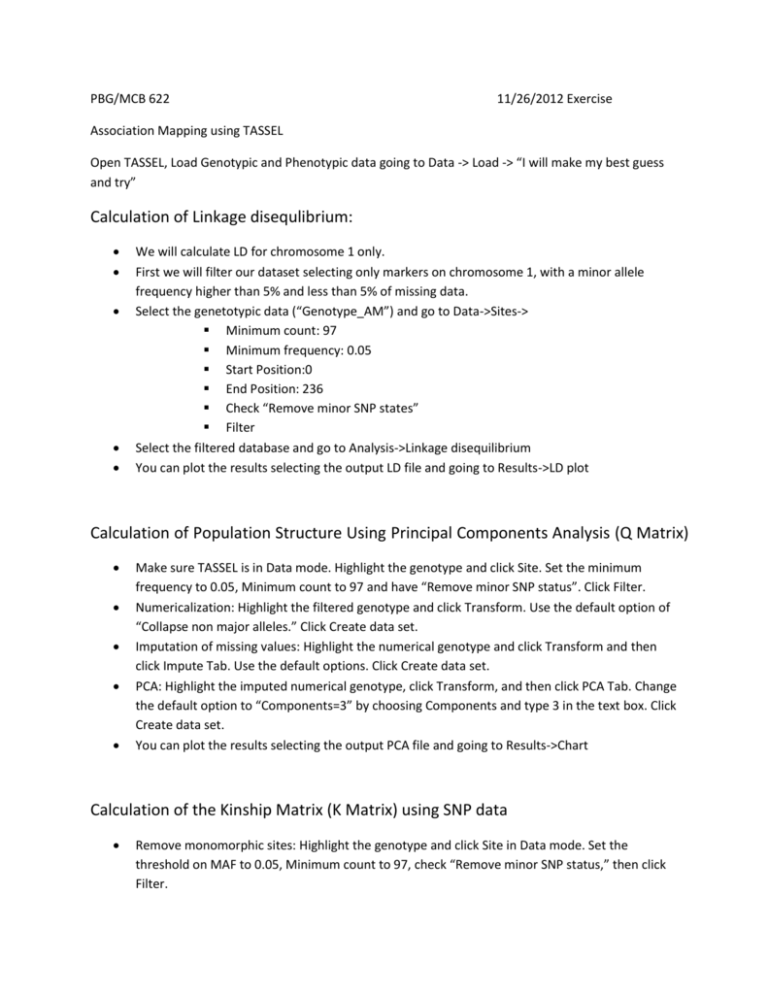
PBG/MCB 622
11/26/2012 Exercise
Association Mapping using TASSEL
Open TASSEL, Load Genotypic and Phenotypic data going to Data -> Load -> “I will make my best guess
and try”
Calculation of Linkage disequlibrium:





We will calculate LD for chromosome 1 only.
First we will filter our dataset selecting only markers on chromosome 1, with a minor allele
frequency higher than 5% and less than 5% of missing data.
Select the genetotypic data (“Genotype_AM”) and go to Data->Sites->
 Minimum count: 97
 Minimum frequency: 0.05
 Start Position:0
 End Position: 236
 Check “Remove minor SNP states”
 Filter
Select the filtered database and go to Analysis->Linkage disequilibrium
You can plot the results selecting the output LD file and going to Results->LD plot
Calculation of Population Structure Using Principal Components Analysis (Q Matrix)





Make sure TASSEL is in Data mode. Highlight the genotype and click Site. Set the minimum
frequency to 0.05, Minimum count to 97 and have “Remove minor SNP status”. Click Filter.
Numericalization: Highlight the filtered genotype and click Transform. Use the default option of
“Collapse non major alleles.” Click Create data set.
Imputation of missing values: Highlight the numerical genotype and click Transform and then
click Impute Tab. Use the default options. Click Create data set.
PCA: Highlight the imputed numerical genotype, click Transform, and then click PCA Tab. Change
the default option to “Components=3” by choosing Components and type 3 in the text box. Click
Create data set.
You can plot the results selecting the output PCA file and going to Results->Chart
Calculation of the Kinship Matrix (K Matrix) using SNP data

Remove monomorphic sites: Highlight the genotype and click Site in Data mode. Set the
threshold on MAF to 0.05, Minimum count to 97, check “Remove minor SNP status,” then click
Filter.

Estimate kinship: Highlight the filtered genotype and click Kinship in Data mode. A kinship matrix
will be added to the data tree under Matrix category.
Association analysis using GLM (Least squares fixed effects linear model)
1) Naïve Model: Flowering time = Marker effect + residual




Remove monomorphic sites: Highlight the genotype and click Site in Data mode. Set the
threshold on MAF as 0.05, Minimum count to 97, then click Filter.
Joining data: Highlight the two data sets (Filtered genotype and phenotype) by holding the
Control key while selecting the individual data. Then click Intersection (∩) Join on Data mode to
create a combined data set.
Association analysis: Highlight the joint data set then click GLM in Analysis mode to perform
association analysis. Two reports will be added to the data tree.
Visualize results by selecting the “GLM_Marker_test” results file and clicking Results->
Manhattan Plot
2) Q Model: Flowering time = Population Structure+Marker effect + residual




Remove monomorphic sites: Highlight the genotype and click Site in Data mode. Set the
threshold on MAF as 0.05, Minimum count to 97, then click Filter.
Joining data: Highlight the three filtered data sets (“PC_genotype_for_AM”, Filtered genotype
and phenotype) by holding the Control key while selecting the individual data. Then click
Intersection (∩) Join on Data mode to create a combined data set.
Association analysis: Highlight the joint data set then click GLM in Analysis mode to perform
association analysis. Two reports will be added to the data tree.
Visualize results by selecting the “GLM_Marker_test” results file and clicking Results->
Manhattan Plot
Association analysis using MLM (Mixed linear model: Individuals and the residual
are fit as random effects. The other terms are treated as fixed effects.)
3) Q+K Model: Flowering time = Population Structure+ Marker effect + Individuals + residual


Association analysis: Highlight the joint data set created for the Q model
(Phenotype+genotype+PCA) and the Kinship Matrix. Click MLM in Analysis mode. Apply all the
default settings.
Visualize results by selecting the “GLM_Marker_test” results file and clicking Results->
Manhattan Plot