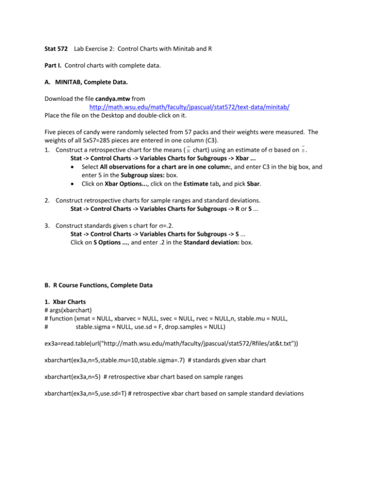
Stat 572 Lab Exercise 2: Control Charts with Minitab and R
Part I. Control charts with complete data.
A. MINITAB, Complete Data.
Download the file candya.mtw from
http://math.wsu.edu/math/faculty/jpascual/stat572/text-data/minitab/
Place the file on the Desktop and double-click on it.
Five pieces of candy were randomly selected from 57 packs and their weights were measured. The
weights of all 5x57=285 pieces are entered in one column (C3).
1. Construct a retrospective chart for the means ( x chart) using an estimate of  based on s .
Stat -> Control Charts -> Variables Charts for Subgroups -> Xbar ...
 Select All observations for a chart are in one column:, and enter C3 in the big box, and
enter 5 in the Subgroup sizes: box.
 Click on Xbar Options..., click on the Estimate tab, and pick Sbar.
2. Construct retrospective charts for sample ranges and standard deviations.
Stat -> Control Charts -> Variables Charts for Subgroups -> R or S ...
3. Construct standards given s chart for =.2.
Stat -> Control Charts -> Variables Charts for Subgroups -> S ...
Click on S Options ..., and enter .2 in the Standard deviation: box.
B. R Course Functions, Complete Data
1. Xbar Charts
# args(xbarchart)
# function (xmat = NULL, xbarvec = NULL, svec = NULL, rvec = NULL,n, stable.mu = NULL,
#
stable.sigma = NULL, use.sd = F, drop.samples = NULL)
ex3a=read.table(url("http://math.wsu.edu/math/faculty/jpascual/stat572/Rfiles/at&t.txt"))
xbarchart(ex3a,n=5,stable.mu=10,stable.sigma=.7) # standards given xbar chart
xbarchart(ex3a,n=5) # retrospective xbar chart based on sample ranges
xbarchart(ex3a,n=5,use.sd=T) # retrospective xbar chart based on sample standard deviations
2. R Charts
# args(rchart)
# function (xmat = NULL, rvec = NULL, n, stable.sigma = NULL, drop.samples = NULL)
rchart(ex3a,n=5,stable.sigma=.7) # standards given R chart with complete data
rchart(ex3a,n=5) # retrospective R chart with complete data
# standards given R chart with probability limits and complete data
RPLchart(ex3a,n=5,stable.sigma=.7,alpha=.005)
# Probability Limits
# args(RPLchart)
# function (xmat = NULL, rvec = NULL, n, stable.sigma = NULL, drop.samples = NULL,
alpha = 0.005)
RPLchart(ex3a,n=5,alpha=.005) # retrospective R chart with probability limits and complete data
3. s Charts
# args(schart)
# function (xmat = NULL, svec = NULL, n, stable.sigma = NULL, drop.samples = NULL)
schart(ex3a,n=5,stable.sigma=.7) # standards given s chart with complete data
schart(ex3a,n=5) # retrospective s chart with complete data
# Probability Limits
# args(sPLchart)
# function (xmat = NULL, svec = NULL, n, stable.sigma = NULL, drop.samples = NULL,
#
alpha)
# standards given s chart with probability limits and complete data
sPLchart(ex3a,n=5,stable.sigma=.7,alpha=.005)
sPLchart(ex3a,n=5,alpha=.005) # retrospective s chart with probability limits and complete data
C. Charts with Dropped Samples
# Use the option drop.samples to identify samples that you want excluded from the charts.
# s and xbar charts with samples 10 and 18 deleted
par(mfrow=c(2,1))
schart(ex3a,n=5,drop.samples=c(10,18)) # retro s chart
xbarchart(ex3a,n=5,use.sd=F,drop.samples=c(10,18)) # retro xbar chart
par(mfrow=c(1,1))
Part II. Control charts when only summary data are available.
I recommend using R instead of Minitab in this case. Use the course R functions.
A. Xbar Chart when Only Values of x Are Given:
# standards given xbar chart
xbarchart(xbarvec=c(10.44,10.46,9.98,9.82,10.90,10.36,11.32,10.86,10.58,9.52,10.56,9.96,10.44,10.96,1
1.14,10.04,11.44,11.84,11.14,11.44),n=5,stable.mu=10,stable.sigma=.7)
# retrospective xbar chart based on ranges
xbarchart(xbarvec=c(10.44,10.46,9.98,9.82,10.90,10.36,11.32,10.86,10.58,9.52,10.56,9.96,10.44,10.96,1
1.14,10.04,11.44,11.84,11.14,11.44),n=5,rvec=c(1.8,1.4,.7,2.6,2.4,1.1,0.8,1.2,.5,1.9,1.5,2.4,2.8,1,1.5,.8,2.
1,1.,2.7,1.6))
B. R Charts when Only Values of R Are Given:
# standards given R chart, given only sample ranges
rchart(rvec=c(1.8,1.4,.7,2.6,2.4,1.1,0.8,1.2,.5,1.9,1.5,2.4,2.8,1,1.5,.8,2.1,1.,2.7,1.6),n=5,stable.sigma=.7)
RPLchart(rvec=c(1.8,1.4,.7,2.6,2.4,1.1,0.8,1.2,.5,1.9,1.5,2.4,2.8,1,1.5,.8,2.1,1.,2.7,1.6),n=5,stable.sigma=.7,alpha=.0005)
# retrospective R chart, given only sample ranges
rchart(rvec=c(1.8,1.4,.7,2.6,2.4,1.1,0.8,1.2,.5,1.9,1.5,2.4,2.8,1,1.5,.8,2.1,1.,2.7,1.6),n=5)
RPLchart(rvec=c(1.8,1.4,.7,2.6,2.4,1.1,0.8,1.2,.5,1.9,1.5,2.4,2.8,1,1.5,.8,2.1,1.,2.7,1.6),n=5,alpha=.0005)
C. s Charts when Only Values of s are Given
# standards given s chart, given only sample standard deviations
schart(svec=c(.8,.5,.45,.9),n=4,stable.sigma=.4)