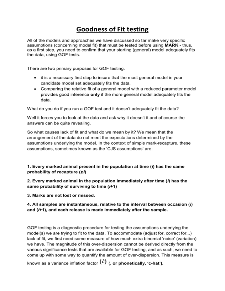
Goodness of Fit testing
All of the models and approaches we have discussed so far make very specific
assumptions (concerning model fit) that must be tested before using MARK - thus,
as a first step, you need to confirm that your starting (general) model adequately fits
the data, using GOF tests.
There are two primary purposes for GOF testing.


it is a necessary first step to insure that the most general model in your
candidate model set adequately fits the data.
Comparing the relative fit of a general model with a reduced parameter model
provides good inference only if the more general model adequately fits the
data.
What do you do if you run a GOF test and it doesn’t adequately fit the data?
Well it forces you to look at the data and ask why it doesn’t it and of course the
answers can be quite revealing.
So what causes lack of fit and what do we mean by it? We mean that the
arrangement of the data do not meet the expectations determined by the
assumptions underlying the model. In the context of simple mark-recapture, these
assumptions, sometimes known as the ‘CJS assumptions’ are:
1. Every marked animal present in the population at time (i) has the same
probability of recapture (pi)
2. Every marked animal in the population immediately after time (i) has the
same probability of surviving to time (i+1)
3. Marks are not lost or missed.
4. All samples are instantaneous, relative to the interval between occasion (i)
and (i+1), and each release is made immediately after the sample.
GOF testing is a diagnostic procedure for testing the assumptions underlying the
model(s) we are trying to fit to the data. To accommodate (adjust for, correct for...)
lack of fit, we first need some measure of how much extra binomial ‘noise’ (variation)
we have. The magnitude of this over-dispersion cannot be derived directly from the
various significance tests that are available for GOF testing, and as such, we need to
come up with some way to quantify the amount of over-dispersion. This measure is
known as a variance inflation factor
(, or phonetically, ‘c-hat’).
C-hat is the measure of the lack of fit between the general and saturated models and
so as the general model gets ‘further away’ from the saturated model, c-hat >1. Now
a saturated model is loosely defined as the model where the number of parameters
equals the number of data points - as such, the fit of the saturated model to the data
is effectively ’perfect’ (or, as good as it’s going to get).
Many different approaches to estimating this are available and you can find a full
description of this in Chapter 5 of the MARK book. There are several approaches
you can use including program RELEASE GOF within MARK itself (only applicable
to the recapture model) and the Bootstrap, and median c-hat approaches which
use simulation and re-sampling to generate the estimate of c hat. Rather than
assuming that the distribution of the model deviance is in fact χ2 distributed (since it
generally isn’t, for typical ’MARK data’), the bootstrap and median c-hat
approaches generate the distribution of model deviances, given the data, and
compare the observed value against this generated distribution. The disadvantage of
the bootstrap and median c hat approaches (beyond some technical issues) is that
both merely estimate c hat. While this is useful (in a practical sense), it reveals
nothing about the underlying sources of lack of fit.
Program RELEASE GOF: 2 tests associated with it
Test 2 – tests the assumption that all marked animals are equally detectable
Test 3 - tests the assumption that that all marked animals alive at (i) have the same
probability of surviving to (i+1) - the second CJS assumption.
It is easy to run simply highlight your most parameterised model (e.g. in the dipper
case Phi(t)p(t)) and select RELEASE GOF under the “tests” tab. It will run
automatically and spawn a notepad window. BUT i don’t want you to use this and
if you want to know more then read pages 147-155 (Chp5-9 – Chp 5-17)
POINT TO REMEMBER – USE THESE TESTS ON YOUR MOST GENERAL
MODEL I.E. THE ONE WITH THE MOST PARAMETERS ONLY.
e.g. IN THE DIPPER CASE
Phi(t)p(t).
e.g. IN THE SWIFT CASE
Phi(c*t)p(c*t).
BOOTSTRAP APPROACH.
The bootstrap approach simulates data based on the parameter estimates of the
model and these simulated data exactly meet the assumptions of the model, i.e., no
over-dispersion is included, animals are totally independent, and no violations of
model assumptions are included. Data are simulated based on the number of
animals released at each occasion. So basically the bootstrap will generate a whole
set of deviances, c hat estimates AICc values etc, etc and you would look at where
your model deviance falls in the distribution. So if you ran 100 simulations and your
model fell between the 80 and 81st simulation (when sorted by deviance values from
lowest to highest) you would have an approximation that your model deviance was
reasonably likely to be observed P < 0.19 (19 models with a higher deviance/100).
How many simulations to use? Run 100 simulations, and do a rough comparison of
where the observed deviance falls on the distribution of these 100 values. If the “P
value” is > 0.2, then doing more simulations is probably a waste of time - the results
are unlikely to change much (although obviously the precision of your estimate of the
P-value will improve). However as the value gets closer to nominal significance (say,
if the observed P-value is < 0.2), then it is probably worth doing ≫ 100 simulations
(say, 500 or 1000). Note that this is likely to take a long time (relatively speaking,
depending on the speed of your computer).
To get the bootstrap approach running, simply select this option under the “tests”
tab. You will get a window like this. Click the top option and hit OK.
You will then be asked to name the bootstrap results dbf file
Give it a unique identifier – normally in relation to the dataset and model
concerned - and click save. You will then get a little confirmation window. After this
you will get the following. Now select the number of simulations (start with 100 but
see above) and leave the random number seed at 0. The next time you come to do
this choose a different random number seed e.g. 1, 2 etc.
As stated above the time taken for this to run will vary on the model, number of
simulations and your computer power – so could take a long time.
When completed you need to choose “view simulation results” under the simulations
tab. Choose the appropriate file (the one you just named) and you will get a window
like the following
You can sort the data using the AZ↓ key and choosing which column header to use –
i would use the deviance. You can then check where your model deviance falls in the
distribution. You can also generate summary data from the simulations using the
little calculator key – very useful.
BUT HOW DO I GET MY ESTIMATE OF C HAT?
Either use:
1) Observed deviance /mean deviance of simulations to estimate c hat or
2) Observed model deviance /deviance df will give you an observed model c hat
which you can then divide by the mean of the simulated c hats). You can obtain
the observed model c hat by selecting “median c hat” under the “tests” tab (see
below).
Which one should i choose? I would calculate both and use the higher value of the 2
as this will make your estimates more conservative.
Recently as an alternative the Median c hat approach has been used ( see MARK
book for a full description).
MEDIAN C HAT APPROACH. This gives you an estimate of c hat. Simply select
“median c hat” under the “tests” tab. You will get a window like this which gives you
the observed model deviance /deviance df at the top. This is the observed model
c-hat that you would need in the above.
You should always set the lower bound at 1 and the upper bound at 3. Why these
values? 1 because a c hat =1 would be a perfect fit and if c hat>3 then there is
probably some fundamental problems with your model. I would set the #
intermediate points = 3 and then it is entirely up to you how many replicates you
choose. I would use a 100. Click ok and it will run and then spawn a Notepad
window which will give you an estimate of c hat at the very top + a se. It will also
produce a graph within MARK which will also show the estimate of c hat.
I have my c hat estimates now what do i do?
Well you can adjust your original model estimates (which were based on c-hat =1
and now you can account for some of that over-dispersion). To do this you simply
select the “c hat” option under the “Adjustments” tab and enter your value for c hat.
Once you do this your results browser will change - try typing in 1.5 for the Phi(t)p(t)
model in the male dipper dataset.
This will result in QuasiAICc values and the weighting of your models will also
change. The best fitting model has suddenly become a much better fitting model
compared to the others in this example. If you get estimates for these new adjusted
models you will notice that the parameter estimates are still the same but the
standard errors of those estimates will have changed.
How big a c hat can you use ?
When should you apply a new c hat? Is 1.5 really different than the null, default value
of 1.0? At what point is c hat too large to be useful? If the model fits perfectly, then c
hat = 1. What about if c hat = 2, or c hat = 10? Is there a point of diminishing utility?
As a working “rule of thumb”, provided c hat ≤ 3, you should feel relatively safe.
Above 3 and you need to consider whether your model is adequate.