Web Appendix: Stata code
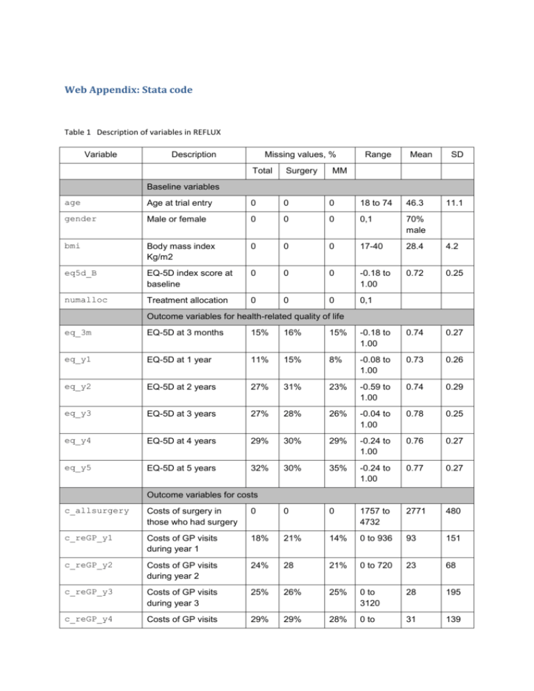
Table 1 Description of variables in REFLUX
Variable
Description
Missing values, %
Total
Surgery
Range
Mean
SD
MM
Baseline variables
age
Age at trial entry
0
0
0
18 to 74
46.3
gender
Male or female
0
0
0
0,1
70%
male
bmi
Body mass index
Kg/m2
0
0
0
17-40
28.4
4.2
eq5d_B
EQ-5D index score at
baseline
0
0
0
-0.18 to
1.00
0.72
0.25
numalloc
Treatment allocation
0
0
0
0,1
11.1
Outcome variables for health-related quality of life
eq_3m
EQ-5D at 3 months
15%
16%
15%
-0.18 to
1.00
0.74
0.27
eq_y1
EQ-5D at 1 year
11%
15%
8%
-0.08 to
1.00
0.73
0.26
eq_y2
EQ-5D at 2 years
27%
31%
23%
-0.59 to
1.00
0.74
0.29
eq_y3
EQ-5D at 3 years
27%
28%
26%
-0.04 to
1.00
0.78
0.25
eq_y4
EQ-5D at 4 years
29%
30%
29%
-0.24 to
1.00
0.76
0.27
eq_y5
EQ-5D at 5 years
32%
30%
35%
-0.24 to
1.00
0.77
0.27
Outcome variables for costs
c_allsurgery
Costs of surgery in
those who had surgery
0
0
0
1757 to
4732
2771
480
c_reGP_y1
Costs of GP visits
during year 1
18%
21%
14%
0 to 936
93
151
c_reGP_y2
Costs of GP visits
during year 2
24%
28
21%
0 to 720
23
68
c_reGP_y3
Costs of GP visits
during year 3
25%
26%
25%
0 to
3120
28
195
c_reGP_y4
Costs of GP visits
29%
29%
28%
0 to
31
139
Variable
Description
Missing values, %
Total
Surgery
Range
Mean
SD
MM
during year 4
1860
c_reGP_y5
Costs of GP visits
during year 5
31%
29%
34%
0 to
1104
30
114
c_hosp_y1
Costs of
hospitalizations during
year 1
18%
21%
14%
0 to
7028
257
848
c_hosp_y2
Costs of
hospitalizations during
year 2
24%
28%
21%
0 to
3069
45
299
c_hosp_y3
Costs of
hospitalizations during
year 3
25%
26%
25%
0 to
8461
117
646
c_hosp_y4
Costs of
hospitalizations during
year 4
29%
29%
28%
0 to
14117
149
979
c_hosp_y5
Costs of
hospitalizations during
year 5
31%
29%
34%
0 to
3754
85
451
c_drug_y1
Costs of drugs during
year 1
18%
21%
14%
0 to 617
55
91
c_drug_y2
Costs of drugs during
year 2
24%
28%
21%
0 to 719
61
116
c_drug_y3
Costs of drugs during
year 3
25%
26%
25%
0 to 682
55
106
c_drug_y4
Costs of drugs during
year 4
29%
29%
28%
0 to -655
54
103
c_drug_y5
Costs of drugs during
year 5
31%
29%
34%
0 to 655
53
100
Outcomes for cost-effectiveness
total_QALYs
Total QALYs over 5
years*
51%
52%
51%
0.02 to
4.67
3.60
0.95
total_costs
Total costs over 5
years*
46%
47%
46%
0 to
10163
2100
1956
*Total QALYs and total costs over 5 years refer to the sum of QALYs and costs discounted at a 3.5%
annual rate over the individuals with complete data for the relevant variables (EQ-5D for QALYs and
cost components for costs).
Note that data were modified to simplify the illustration of the different methods to handle missing
data.
Stata code using ice
1. Install ice
findit ice//choose the first option on the list. The ‘mim’ package should
also appear on this list.
2. Prepare data for multiple imputation
//calculate discounted costs at each year
gen costs_year1 = c_allsurgery + c_drug_y1
gen costs_year2_D = (c_drug_y2 + c_reGP_y2 +
gen costs_year3_D = (c_drug_y3 + c_reGP_y3 +
gen costs_year4_D = (c_drug_y4 + c_reGP_y4 +
gen costs_year5_D = (c_drug_y5 + c_reGP_y5 +
+ c_reGP_y1 + c_hosp_y1
c_hosp_y2)*(1.035)^(-1)
c_hosp_y3)*(1.035)^(-2)
c_hosp_y4)*(1.035)^(-3)
c_hosp_y5)*(1.035)^(-4)
//calculate discounted QALYs at each year
gen QALY_y1 = ((eq5d_B + eq_3m)/2)*0.25 + ((eq_3m + eq_y1)/2)*0.75
gen QALY_y2= ((eq_y1 + eq_y2)/2)*(1.035)^(-1)
gen QALY_y3= ((eq_y2+eq_y3)/2)*(1.035)^(-2)
gen QALY_y4= ((eq_y3+eq_y4)/2)*(1.035)^(-3)
gen QALY_y5= ((eq_y4+eq_y5)/2)*(1.035)^(-4)
//NB we could equally well apply the discounting after imputing
keep studyno eq5d_B QALY_y1 QALY_y2 QALY_y3 QALY_y4 QALY_y5 costs_year1
costs_year2_D /*
*/ costs_year3_D costs_year4_D costs_year5_D numalloc bmi age gender
3. Multiple imputation with chained equations using ice
ice eq5d_B QALY_y1 QALY_y2 QALY_y3 QALY_y4 QALY_y5 /*
*/ costs_year1 costs_year2_D costs_year3_D costs_year4_D costs_year5_D /*
*/ numalloc bmi age gender, saving(MI_aggregated, replace) /*
*/ m(60) match genmiss(ind_miss) by(numalloc) seed(10)
/* This command runs multiple imputation with chained equations using the
models shown in Figure 1 below and saves the multiple imputed dataset in
‘MI_aggregated’. The multiple imputation generates 60 (m=60) datasets using
predictive mean matching (‘match’) and separately by treatment allocation
(‘by(numalloc)’). ‘genmiss’ generates an indicator of missingness; =1 if
observation was originally missing or =0 otherwise. ‘seed’ sets a random
number seed, which is useful to improve consistency across imputations. */
use MI_aggregated, clear //open multiple imputed dataset
//generate total QALYs and total costs
gen total_QALYs = QALY_y1 + QALY_y2 + QALY_y3 + QALY_y4 + QALY_y5
gen total_costs = costs_year1 + costs_year2_D + costs_year3_D +
costs_year4_D + costs_year5_D
drop if _mj==0 //this is the original dataset with missing data
//obtain average total costs and QALYs per patient
mim: mean total_costs total_QALYs, over(numalloc)
//convert data into Stata mi estimate format
mi import ice, clear
Figure 1 Prediction equations generated from the ice command
Variable
Command
eq5d_B
numalloc
bmi
age
gender
costs_year1
regress
QALY_y1
regress
costs_y~2_D
regress
costs_y~3_D
regress
QALY_y2
regress
costs_y~4_D
regress
costs_y~5_D
regress
QALY_y4
regress
QALY_y3
regress
QALY_y5
regress
Prediction equation
[No missing data in estimation sample]
[No missing data in estimation sample]
[No missing data in estimation sample]
[No missing data in estimation sample]
[No missing data in estimation sample]
eq5d_B QALY_y1 QALY_y2 QALY_y3 QALY_y4 QALY_y5
costs_year2_D costs_year3_D costs_year4_D
costs_year5_D numalloc bmi age gender
eq5d_B QALY_y2 QALY_y3 QALY_y4 QALY_y5 costs_year1
costs_year2_D costs_year3_D costs_year4_D
costs_year5_D numalloc bmi age gender
eq5d_B QALY_y1 QALY_y2 QALY_y3 QALY_y4 QALY_y5
costs_year1 costs_year3_D costs_year4_D costs_year5_D
numalloc bmi age gender
eq5d_B QALY_y1 QALY_y2 QALY_y3 QALY_y4 QALY_y5
costs_year1 costs_year2_D costs_year4_D costs_year5_D
numalloc bmi age gender
eq5d_B QALY_y1 QALY_y3 QALY_y4 QALY_y5 costs_year1
costs_year2_D costs_year3_D costs_year4_D
costs_year5_D numalloc bmi age gender
eq5d_B QALY_y1 QALY_y2 QALY_y3 QALY_y4 QALY_y5
costs_year1 costs_year2_D costs_year3_D costs_year5_D
numalloc bmi age gender
eq5d_B QALY_y1 QALY_y2 QALY_y3 QALY_y4 QALY_y5
costs_year1 costs_year2_D costs_year3_D costs_year4_D
numalloc bmi age gender
eq5d_B QALY_y1 QALY_y2 QALY_y3 QALY_y5 costs_year1
costs_year2_D costs_year3_D costs_year4_D
costs_year5_D numalloc bmi age gender
eq5d_B QALY_y1 QALY_y2 QALY_y4 QALY_y5 costs_year1
costs_year2_D costs_year3_D costs_year4_D
costs_year5_D numalloc bmi age gender
eq5d_B QALY_y1 QALY_y2 QALY_y3 QALY_y4 costs_year1
costs_year2_D costs_year3_D costs_year4_D
costs_year5_D numalloc bmi age gender
4. Multiple imputation with chained equations using mi impute chained
misstable summ, gen(M_) //reports counts of missing values and create an
indicator variable for missingness
mi set wide //register dataset to be imputed
mi register imputed costs_year1 costs_year2_D costs_year3_D costs_year4_D
costs_year5_D //cost variables to be imputed
mi register imputed QALY_y1 QALY_y2 QALY_y3 QALY_y4 QALY_y5 //QALY
variables to be imputed
mi register regular numalloc bmi age gender eq5d_B //regular variables that
do not require imputation
mi impute chained (pmm) QALY_y1 QALY_y2 QALY_y3 /*
*/ QALY_y4 QALY_y5 costs_year1 costs_year2_D costs_year3_D /*
*/ costs_year4_D costs_year5_D = eq5d_B bmi age gender, add(60)
by(numalloc) rseed(10)
//runs multiple imputation with chained equations with predictive mean
matching (pmm) over 60 (add) imputations by treatment group, setting seed
at 10 (rseed)
mi passive: gen total_QALYs = QALY_y1 + QALY_y2 + QALY_y3 + QALY_y4 +
QALY_y5 //create variable for total QALYs
mi passive: gen total_costs = costs_year1 + costs_year2_D + costs_year3_D
+ costs_year4_D + costs_year5_D // create variable for total costs
Figure 2 Prediction equations generated from the mi impute chained command
Performing setup for each by() group:
-> numalloc = Medical
Conditional models:
costs_year1: pmm costs_year1 QALY_y1 costs_year2_D QALY_y2 costs_year3_D costs_year4_D
QALY_y3 costs_year5_D QALY_y4 QALY_y5 eq5d_B bmi age gender
QALY_y1: pmm QALY_y1 costs_year1 costs_year2_D QALY_y2 costs_year3_D costs_year4_D
QALY_y3 costs_year5_D QALY_y4 QALY_y5 eq5d_B bmi age gender
costs_year2_D: pmm costs_year2_D costs_year1 QALY_y1 QALY_y2 costs_year3_D costs_year4_D
QALY_y3 costs_year5_D QALY_y4 QALY_y5 eq5d_B bmi age gender
QALY_y2: pmm QALY_y2 costs_year1 QALY_y1 costs_year2_D costs_year3_D costs_year4_D
QALY_y3 costs_year5_D QALY_y4 QALY_y5 eq5d_B bmi age gender
costs_year3_D: pmm costs_year3_D costs_year1 QALY_y1 costs_year2_D QALY_y2 costs_year4_D
QALY_y3 costs_year5_D QALY_y4 QALY_y5 eq5d_B bmi age gender
costs_year4_D: pmm costs_year4_D costs_year1 QALY_y1 costs_year2_D QALY_y2 costs_year3_D
QALY_y3 costs_year5_D QALY_y4 QALY_y5 eq5d_B bmi age gender
QALY_y3: pmm QALY_y3 costs_year1 QALY_y1 costs_year2_D QALY_y2 costs_year3_D
costs_year4_D costs_year5_D QALY_y4 QALY_y5 eq5d_B bmi age gender
costs_year5_D: pmm costs_year5_D costs_year1 QALY_y1 costs_year2_D QALY_y2 costs_year3_D
costs_year4_D QALY_y3 QALY_y4 QALY_y5 eq5d_B bmi age gender
QALY_y4: pmm QALY_y4 costs_year1 QALY_y1 costs_year2_D QALY_y2 costs_year3_D
costs_year4_D QALY_y3 costs_year5_D QALY_y5 eq5d_B bmi age gender
QALY_y5: pmm QALY_y5 costs_year1 QALY_y1 costs_year2_D QALY_y2 costs_year3_D
costs_year4_D QALY_y3 costs_year5_D QALY_y4 eq5d_B bmi age gender
5. Analysis of multiple imputed datasets (post ice or mi impute chained)
//Regress using seemingly unrelated regression (SUR)
xi: mi estimate, cmdok: sureg (total_cost numalloc) (total_QALY numalloc
eq5d_B), corr
//Probability of cost-effectiveness using coefficients from SUR
matrix beta = e(b_mi)
// extract coefficients
matrix vari = e(V_mi)
// extract variance-covariance matrix
scalar QD = beta[1,3]
// difference in QALYs
scalar CD = beta[1,1]
// difference in costs
scalar varQD= vari[3,3]
// variance for QALYs
scalar varCD = vari[1,1]
// variance for costs
scalar cov = vari[3,1]
// covariance
di “ICER=” CD/QD
di “Prob cost-effective=” normal((20000*QD-CD)/sqrt((20000)^2 * varQD +
varCD - 2*20000*cov))
//Probability of cost-effectiveness using bootstrap (alternative to SUR)
cap prog drop misim
program define misim, rclass
version 10.1
mim: reg total_QALYs numalloc eq5d_B
matrix define Q = e(MIM_Q)
return scalar q1 = Q[1,1]
mim: reg total_costs numalloc
matrix define C = e(MIM_Q)
return scalar c1 = C[1,1]
end
keep
studyno numalloc eq5d_B total_QALYs total_costs _mi _mj
//Bootstrap
bootstrap q1=r(q1) c1=r(c1), rep(1000) cluster(_mi) strata (numalloc)/*
*/ saving (bootstrap_MIA, replace): misim
use bootstrap_MIA, clear //use dataset with coefficients from bootstrap
summ q1 c1 //return the average incremental QALYs (q1) and costs (c1)
//Calculate probability that surgery is cost-effective for each threshold
local c = 0
forvalues l=0(1000)40000 {
local c = `c'+1
gen l`c' = `l'
gen p`c'=cond(`l'*q1>=c1,1,0)
}
keep l* p*
collapse (mean) l* p*
gen temp = 1
reshape long l p, i(temp) j(id)
drop temp
//Display probability at a threshold of 20,000/QALY
list p if l==20000
6. Mixed effects model
//generate total costs and QALYs - note that in this example, the
discounting is done after the analysis
gen cost1 = (c_allsurgery + c_drug_y1 + c_reGP_y1 + c_hosp_y1) / 1000
gen cost2= (c_drug_y2 + c_reGP_y2 + c_hosp_y2) / 1000
gen cost3 = (c_drug_y3 + c_reGP_y3 + c_hosp_y3) / 1000
gen cost4 = (c_drug_y4 + c_reGP_y4 + c_hosp_y4) / 1000
gen cost5 = (c_drug_y5 + c_reGP_y5 + c_hosp_y5) / 1000
// costs are scaled down by 1000 to transform them into a similar scale as
QALYs
gen
gen
gen
gen
gen
QALY1 = ((eq5d_B + eq_3m)/2)*0.25 + ((eq_3m + eq_y1)/2)*0.75
QALY2= (eq_y1 + eq_y2)/2
QALY3= (eq_y2+eq_y3)/2
QALY4= (eq_y3+eq_y4)/2
QALY5= (eq_y4+eq_y5)/2
//keep variables required for the analysis
keep studyno numalloc cost* QALY* age bmi gender eq5d_B
drop cost_drug*
//reshape from wide to long creating a new variable - year - that indicates
time period
reshape long cost QALY, i(studyno) j(year)
label val year
//reshape again to create a single dependent variable - y. The variable
type indicates whether it refers to costs or QALYs
rename cost y1
rename QALY y2
reshape long y, i(studyno year) j(type)
gen cost=type==1
gen QALY=type==2
egen yeartype=group(year type)
//Mixed model
xtmixed y i.cost#i.year i.cost#i.numalloc#i.year i.cost#i.year#c.eq5d_B ||
studyno: /*
*/ , nocons ||, res(uns, t(yeartype)) remlemiterate(100) emtolerance(1e-5)
/*i.cost#i.year represents the interaction between the cost and QALYs and
each time point; i.cost#i.numalloc#i.year represents the effect of
treatment (numalloc) on costs and QALYs at each time point;
i.cost#i.year#c.eq5d_B represents the effect of EQ-5D at baseline on costs
and QALYs at each time point.
// scale cost coefficients up and estimate discounted treatment effect on
costs and QALYs
local scale_up = 1000
local discount1 = (1.035)^-1
local discount2 = (1.035)^-2
local discount3 = (1.035)^-3
local discount4 = (1.035)^-4
nlcom (Dcost: `scale_up' * _b[1.cost#1.numalloc#1.year]
treatment effect on costs
/// discounted
+
+
+
+
(DQALY:
QALYs
+
+
+
+
`scale_up' * `discount1' * _b[1.cost#1.numalloc#2.year] ///
`scale_up' * `discount2' * _b[1.cost#1.numalloc#3.year] ///
`scale_up' * `discount3' * _b[1.cost#1.numalloc#4.year] ///
`scale_up' * `discount4' * _b[1.cost#1.numalloc#5.year]) ///
_b[0.cost#1.numalloc#1.year] /// discounted treatment effect on
`discount1'
`discount2'
`discount3'
`discount4'
*
*
*
*
_b[0.cost#1.numalloc#2.year] ///
_b[0.cost#1.numalloc#3.year] ///
_b[0.cost#1.numalloc#4.year] ///
_b[0.cost#1.numalloc#5.year])
// Probability that intervention is cost-effective as per point 2
matrix beta = r(b)
matrix vari = r(V)
scalar QD = beta[1,2]
scalar CD = beta[1,1]
scalar varQD = vari[2,2]
scalar varCD = vari[1,1]
scalar cov = vari[2,1]
di “ICER=” CD/QD
di “Prob cost-effective=” normal((20000*QD-CD)/sqrt((20000)^2 * varQD +
varCD - 2*20000*cov))
7. Sensitivity analysis – simple approach
Exemplified here with reducing QALYs of all individuals with missing data post ice
use MI_aggregated, clear //open multiple imputed dataset
drop if _mj==0
//The objective is to plot the % change in costs and QALYs on probability
that surgery is cost-effective
// 1. Reduce imputed QALYs by 10% in year 2 to 5
local qalys "QALY_y2 QALY_y3 QALY_y4 QALY_y5 "
foreach var of local qalys {
replace `var'=`var'*0.9 if ind_miss`var'==1
}
// 2. Create new imputed QALYs for year 1
forvalues i=50(10)90{
gen new_QALY_y1_`i'= QALY_y1*`i'/100 if ind_missQALY_y1==1
replace new_QALY_y1_`i' = QALY_y1 if ind_missQALY_y1==0
gen t_QALY`i' = new_QALY_y1_`i' + QALY_y2 + QALY_y3 + QALY_y4 +
}
//3. Calculate total costs
gen total_costs = costs_year1 + costs_year2_D + costs_year3_D +
costs_year4_D + costs_year5_D
QALY_y5
keep t_QALY90 t_QALY80 t_QALY70 t_QALY60 t_QALY50 numalloc eq5d_B _mi _mj
total_cost
//4. run analysis for each
mi import ice, clear
local qalys "t_QALY90 t_QALY80 t_QALY70 t_QALY60 t_QALY50"
foreach var of local qalys {
xi: mi estimate, cmdok: sureg (total_cost numalloc) (`var' numalloc
eq5d_B), corr
matrix beta = e(b_mi)
// extract coefficients
matrix vari = e(V_mi)
// extract var-covar matrix
scalar QD
= beta[1,3]
// difference in QALYs
scalar CD
= beta[1,1]
// difference in costs
scalar varQD
= vari[3,3]
// variance for QALYs
scalar varCD
= vari[1,1]
// variance for costs
scalar cov
= vari[3,1]
// covariance
scalar `var'= normal((20000*QD-CD)/sqrt((20000)^2 * varQD + varCD 2*20000*cov))
}
scalar list t_QALY90 t_QALY80 t_QALY70 t_QALY60 t_QALY50
//probability that intervention is cost-effective at different reductions
of imputed QALYs