Chapter 06 - Multiple Linear Regression Analysis
CHAPTER 6
Answers to End of Chapter Problems
6.1
a. The correlations we are most interested in are those against college GPA because that
is the dependent variable. Hours studied has the highest correlation, then SAT score, and
lastly HS GPA. All of the independent variables are positively and relatively strongly
related to college GPA. We can also see that high-school GPA and hours studied have a
positive and somewhat strong relationship with each other and high-school GPA and
SAT score and SAT score and hours studied have a positive but not as strong
relationship.
b. The correlation matrix sheds light on linear relationships but does offer information on
the marginal effects such as the effect that hours studied has on College GPA holding
SAT score and high-school GPA constant.
6.2
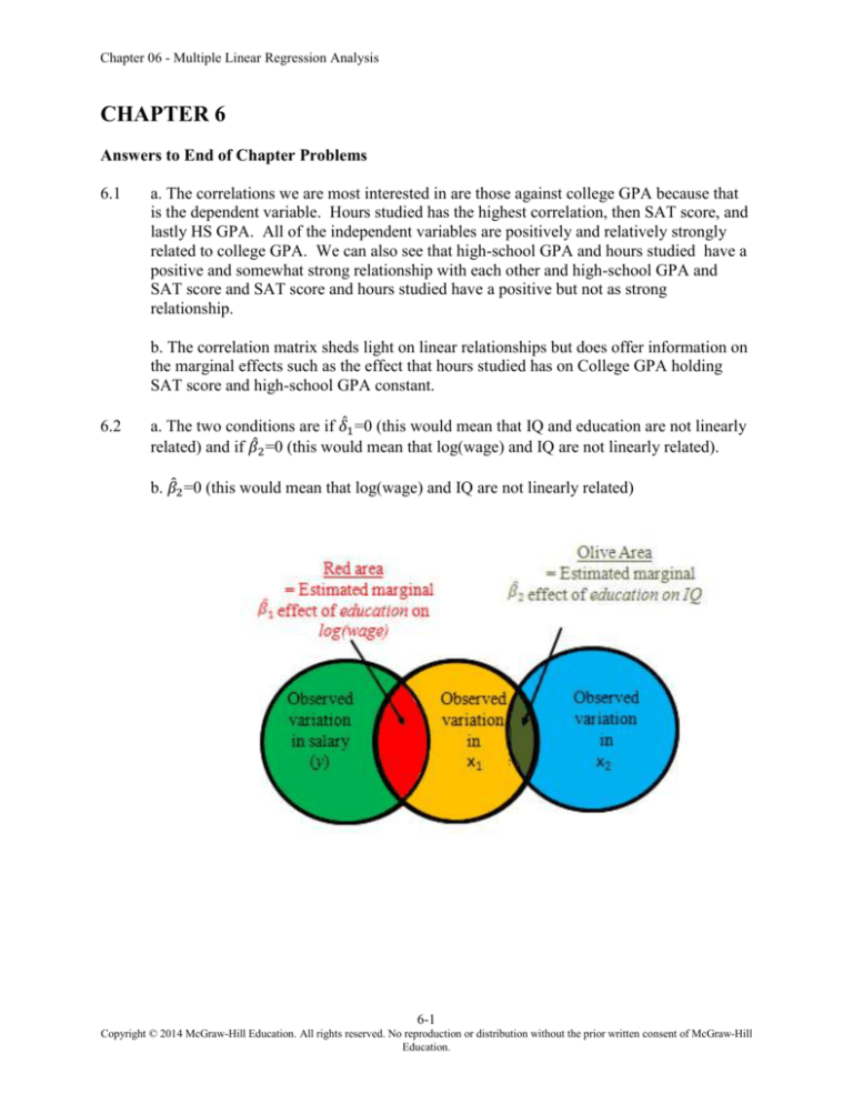
a. The two conditions are if 𝛿̂1 =0 (this would mean that IQ and education are not linearly
related) and if 𝛽̂2=0 (this would mean that log(wage) and IQ are not linearly related).
b. 𝛽̂2=0 (this would mean that log(wage) and IQ are not linearly related)
6-1
Copyright © 2014 McGraw-Hill Education. All rights reserved. No reproduction or distribution without the prior written consent of McGraw-Hill
Education.
Chapter 06 - Multiple Linear Regression Analysis
𝛿̂1 =0 (this would mean that IQ and education are not linearly related)
c. It is genearlly the case the IQ and education are related to each other and IQ is related
to log(wage)
6-2
Copyright © 2014 McGraw-Hill Education. All rights reserved. No reproduction or distribution without the prior written consent of McGraw-Hill
Education.
Chapter 06 - Multiple Linear Regression Analysis
6.3
a. I would expect 𝛽̂1 = 𝛽̃1
b. Again, I would expect 𝛽̂1 = 𝛽̃1
6.4
I would advise my friend that it would be easiest to just regress y on x and z and perform
a t-test on the coefficient on z. The method that the friend suggested is not quite right.
The friend should regress z on x and save the residuals and then regress y on those
residuals. This will give your friend the same results as the first method but the standard
errors of the second method will be wrong.
6-3
Copyright © 2014 McGraw-Hill Education. All rights reserved. No reproduction or distribution without the prior written consent of McGraw-Hill
Education.
Chapter 06 - Multiple Linear Regression Analysis
6.5
a.
b. R-squared is 1,237,904/2,347,829 = .5273. This means that 52.73% of the variation of
Sales is related to advertising, bonus, relative price, and competition.
c. 100%
d. Hypothesis:
𝐻0 : 𝛽1 = 𝛽2 = 𝛽3 = 𝛽4 = 0
𝐻1 : 𝑎𝑡 𝑙𝑒𝑎𝑠𝑡 𝑜𝑛𝑒 𝛽𝑖 𝑖𝑠 𝑛𝑜𝑡 𝑒𝑞𝑢𝑎𝑙 𝑡𝑜 0
Test Statistic
F-statistic = 12.5471 and the p-value of the F-test is 0.001.
Rejection Rule
Reject H0 if the p-value < 0.01.
Rejection Rule
Because 0.001< 0.01 we reject H0 and conclude that at least one of
advertising, bonus, relative price, and competition is related to sales at the
1% level.
e. Bonus
Hypothesis:
𝐻0 : 𝛽2 = 0
𝐻1 : 𝛽2 ≠ 0
Test Statistic
t-statistic = 11.6/3.02= 3.84 and the p-value of the t-test is 0.003.
Rejection Rule
Reject H0 if the p-value < 0.01.
Rejection Rule
Because 0.003 < 0.01 we reject H0 and conclude that bonus is statistically
significant at the 1% level.
f. ADV: On average, holding bonus, relative price, and competition constant, if the
amount spend on advertising increases by $1000, then sales go up by $10,800.
Bonus: On average, holding advertising, relative price, and competition constant, if the
amount spend on bonuses increases by $1000, then sales go up by $11,600.
RELPRICE: On average, holding advertising, bonus, relative price, and competition
constant, if the Medicorp’s relative price increases by $1, then sales goes down by
122,000.
6-4
Copyright © 2014 McGraw-Hill Education. All rights reserved. No reproduction or distribution without the prior written consent of McGraw-Hill
Education.
Chapter 06 - Multiple Linear Regression Analysis
g. The 95% confidence interval is
𝛽̂2 ± 𝑡𝛼,𝑛−𝑘−1 𝑠𝑒𝛽̂2
2
11.6 ± (2.02) (3.02)
(5.5, 17.7)
This interval does not include 0, which means that Bonus is statistically significant at the
5% level.
̂ 𝑖 = 𝛽̂0 + 𝛽̂1 𝐴𝑑𝑣𝑖 + 𝛽̂2 𝐵𝑜𝑛𝑢𝑠𝑖 + 𝛽̂3 𝑅𝑒𝑙𝑝𝑟𝑖𝑐𝑒𝑖 + 𝛽̂4 𝐶𝑜𝑚𝑝𝑒𝑡𝑖
h. 𝑆𝑎𝑙𝑒𝑠
̂ 𝑖 = 889.1 + 10.8𝐴𝑑𝑣𝑖 + 11.6𝐵𝑜𝑛𝑢𝑠𝑖 − 122𝑅𝑒𝑙𝑝𝑟𝑖𝑐𝑒𝑖 − 0.18𝐶𝑜𝑚𝑝𝑒𝑡𝑖
𝑆𝑎𝑙𝑒𝑠
̂ 𝑖 = 889.1 + 10.8(60) + 11.6(45) − 122(0.7) − 0.18(100)
𝑆𝑎𝑙𝑒𝑠
̂ 𝑖 = $2,073,520
𝑆𝑎𝑙𝑒𝑠
6.6
a.
b. R-squared is 1,108,892/2,807,27 9.334= .395. This means that 39.5% of the variation
of price is related to speed and charge.
c. Hypothesis:
𝐻0 : 𝛽1 = 𝛽2 = 0
𝐻1 : 𝑎𝑡 𝑙𝑒𝑎𝑠𝑡 𝑜𝑛𝑒 𝛽𝑖 𝑖𝑠 𝑛𝑜𝑡 𝑒𝑞𝑢𝑎𝑙 𝑡𝑜 0
Test Statistic
F-statistic = 6.203 and the p-value of the F-test is 0.0048.
Rejection Rule
Reject H0 if the p-value < 0.01.
Rejection Rule
Because 0.0048< 0.01 we reject H0 and conclude that at least one of speed
or charge is related to price at the 1% level.
d. Speed
Hypothesis:
𝐻0 : 𝛽1 = 0
𝐻1 : 𝛽1 ≠ 0
Test Statistic
t-statistic = 10.1506/14.5019= 0.7 and the p-value of the t-test is 0.003.
Rejection Rule
Reject H0 if the |t-stat| > 2.1.
Rejection Rule
Because 0.7 < 2.1 we fail to reject H0 and conclude that speed is
statistically unrelated to price at the 5% level.
6-5
Copyright © 2014 McGraw-Hill Education. All rights reserved. No reproduction or distribution without the prior written consent of McGraw-Hill
Education.
Chapter 06 - Multiple Linear Regression Analysis
e. Speed: On average, holding charge constant, if the speed increases by 1megahertz
then price go up by $10.15.
Charge: On average, holding speed constant, if the charge increases by one minute then
price go up by $1.63.
f. The 95% confidence interval is
𝛽̂1 ± 𝑡𝛼,𝑛−𝑘−1 𝑠𝑒𝛽̂1
2
10.15 ± (2.1) (14.5)
(-22.19, 42.49)
This interval includes 0, which means that Speed is statistically insignificant at the 5%
level. This interval brackets 𝛽1 .
g. 𝑠𝑦|𝑥 = √89,389 = 298.98.
̂ 𝑖 = 𝛽̂0 + 𝛽̂1 𝑆𝑝𝑒𝑒𝑑𝑖 + 𝛽̂2 𝐶ℎ𝑎𝑟𝑔𝑒𝑖
h. 𝑃𝑟𝑖𝑐𝑒
̂ 𝑖 = 1500.6 + 10.15𝑆𝑝𝑒𝑒𝑑𝑖 + 1.63𝐶ℎ𝑎𝑟𝑔𝑒𝑖
𝑃𝑟𝑖𝑐𝑒
̂ 𝑖 = 1500.6 + 10.15(33) + 1.63(305)
i. 𝑃𝑟𝑖𝑐𝑒
̂ 𝑖 = $2,332.7
𝑃𝑟𝑖𝑐𝑒
6.7
a. On average, holding population within one mile and population beyond one mile
constant, if the number of competitors within one mile goes up by 1 then sales goes
down by $4,200.
b. On average, holding competition within one mile and population beyond one mile
constant, if the population within one mile goes up by 1000 people then sales goes down
by $6,800.
c. On average, holding competition within one mile and population within one mile
constant, if the population beyond one mile goes up by 1000 people then sales goes
down by $2,300.
̂ 𝑖 = 10.1 − 4.2(2) + 6.8(8) + 2.3(13)
d. 𝑆𝑎𝑙𝑒𝑠
̂ 𝑖 = $86,000
𝑆𝑎𝑙𝑒𝑠
6.8
a. R-squared is 3660.74/4190.95= .8735. This means that 87.35% of the variation of risk
is related to age, pressure, and family.
b. 𝑠𝑦|𝑥 = √33.14 = 5.7567. This is the variation left in risk when the effects of age,
pressure and family have been removed.
c. Age: On average, holding pressure and family constant, if the age of a person
increases by one year then risk go up by 1.08 or 1%.
6-6
Copyright © 2014 McGraw-Hill Education. All rights reserved. No reproduction or distribution without the prior written consent of McGraw-Hill
Education.
Chapter 06 - Multiple Linear Regression Analysis
Pressure: On average, holding age and family constant, if the blood pressure of a
person increases by one then risk go up by .25 or .25%.
Family: On average, holding age and pressure constant, if the number of strokes the
person’s parents have had goes up by one then risk goes up by 8.74 or 8.74%.
d. Hypothesis:
𝐻0 : 𝛽1 = 𝛽2 = 𝛽3 = 0
𝐻1 : 𝑎𝑡 𝑙𝑒𝑎𝑠𝑡 𝑜𝑛𝑒 𝛽𝑖 𝑖𝑠 𝑛𝑜𝑡 𝑒𝑞𝑢𝑎𝑙 𝑡𝑜 0
Test Statistic
F-statistic = 36.82 and the p-value of the F-test is 2.06E-07.
Rejection Rule
Reject H0 if the p-value < 0.01.
Rejection Rule
Because 2.06E-07< 0.01 we reject H0 and conclude that at least one of
age, pressure or family is related to price at the 1% level.
e. Pressure
Hypothesis:
𝐻0 : 𝛽2 = 0
𝐻1 : 𝛽2 ≠ 0
Test Statistic
t-statistic = 0.25/0.05= 5.
Rejection Rule
Reject H0 if the |t-stat| > 1.75.
Rejection Rule
Because 5 > 1.75 we reject H0 and conclude that pressure is statistically
significant at the 10% level.
f. The 95% confidence interval is
𝛽̂1 ± 𝑡𝛼,𝑛−𝑘−1 𝑠𝑒𝛽̂1
2
1.08 ± (2.12) (0.17)
(0.72, 1.44)
This interval does not include 0, which means that age is statistically significant at the 5%
level. This interval brackets 𝛽1 .
̂ 𝑖 = 𝛽̂0 + 𝛽̂1 𝐴𝑔𝑒𝑖 + 𝛽̂2 𝑃𝑟𝑒𝑠𝑠𝑢𝑟𝑒𝑖 + 𝛽̂3 𝐹𝑎𝑚𝑖𝑙𝑦𝑖
g. 𝑅𝑖𝑠𝑘
̂ 𝑖 = −91.76 + 1.08𝐴𝑔𝑒𝑖 + 0.25𝑃𝑟𝑒𝑠𝑠𝑢𝑟𝑒𝑖 + 8.74𝐹𝑎𝑚𝑖𝑙𝑦𝑖
𝑅𝑖𝑠𝑘
̂ 𝑖 = −91.76 + 1.08(70) + 0.25(165) + 8.74(1)
𝑅𝑖𝑠𝑘
̂ 𝑖 = 33.83 or their risk of a stroke is 33.83%
𝑅𝑖𝑠𝑘
h. The prediction could be above 100% or below 0%.
6.9
a. On average, holding square footage and niceness constant, if number of bathrooms
increases by one then the price of the house increases by $10,043.
6-7
Copyright © 2014 McGraw-Hill Education. All rights reserved. No reproduction or distribution without the prior written consent of McGraw-Hill
Education.
Chapter 06 - Multiple Linear Regression Analysis
b. Increasing a niceness rating by 2 will increase the value of the house by
(2)(10,042)=$20,084. If it costs $32,500 to increase the niceness rating from 5 to 7 then
when selling a house 20,084/32,500 = .618 or 61.8%.
c. Increasing a niceness rating by 2 will increase the value of the house by
(2)(10,042)=$20,084. If it costs $24,000 to increase the niceness rating from 2 to 4 then
when selling a house 20,084/24,000 = .8368 or 83.68%.
d. From this question we see that it is more expensive to increase the niceness rating from
5 to 7 than it is to increase the niceness rating from 2 to 4 but the way the regression
model is specified these increases change the value of the house by the same amount. It
would be better to specify the model such that increasing the niceness rating has a nonconstant marginal effect on price.
e. 𝑦̂𝑖 = 𝛽̂0 + 𝛽̂1 𝑥1,𝑖 + 𝛽̂2 𝑥2,𝑖 + 𝛽̂3 𝑥3,𝑖
𝑦̂𝑖 = 24.976 + 0.0526𝑥1,𝑖 + 10.043𝑥2,𝑖 + 10.042𝑥3,𝑖
𝑦̂𝑖 = 24.976 + 0.0526(3200) + 10.043(3) + 10.042(3)
̂𝑦𝑖 = $253,551
6.10
a. To test this hypothesis we need to change the regression model to obtain the standard
error.
𝐻0 : 𝛽1 = 𝛽2 or 𝛽1 − 𝛽2 = 0
𝐻1 : 𝛽1 ≠ 𝛽2 or 𝛽1 − 𝛽2 ≠ 0
𝑦𝑖 = 𝛽0 + 𝛽1 𝑥1,𝑖 + 𝛽2 𝑥2,𝑖 + 𝜀
set 𝛽1 − 𝛽2 = 𝜃 and then solve for 𝛽1
𝛽1 = 𝜃 + 𝛽2 and then substitute this equation into the model for 𝛽1
𝑦𝑖 = 𝛽0 + (𝜃 + 𝛽2 )𝑥1,𝑖 + 𝛽2 𝑥2,𝑖 + 𝜀
𝑦𝑖 = 𝛽0 + 𝜃𝑥1,𝑖 + 𝛽2 𝑥1,𝑖 + 𝛽2 𝑥2,𝑖 + 𝜀
𝑦𝑖 = 𝛽0 + 𝜃𝑥1,𝑖 + 𝛽2 (𝑥1,𝑖 + 𝑥2,𝑖 ) + 𝜀
This equation says that we need to create a new variable, (𝑥1,𝑖 + 𝑥2,𝑖 ), and
the regress 𝑦𝑖 on 𝑥1,𝑖 and (𝑥1,𝑖 + 𝑥2,𝑖 ). The coefficient estimate on 𝑥1,𝑖 is 𝜃̂
and then the standard error on 𝑥1,𝑖 is the standard error of 𝜃̂. The t-stat
next to 𝑥1,𝑖 is the t-stat for the hypothesis and the p-value on 𝑥1,𝑖 is the pvalue for this hypothesis. The rejection rule is to reject H0 if the p-value <
0.05.
b. To generate a confidence interval around a prediction we need to
change the data. We need to create two new columns in Excel. The first
column is generated by taking each 𝑥1 and subtract off 6 (the value of the
prediction for 𝑥1 ) for observations 1 all the way to n and name it (𝑥1 − 6).
The second column is generated by taking each 𝑥2 and subtract off 12 (the
value of the prediction for 𝑥2 ) for observations 1 all the way to n and name
it (𝑥2 − 12). Once these two new columns are created then you need to
regress y on (𝑥1 − 6) and (𝑥2 − 12). The predicted value is the coefficient
estimate next to the intercept, the standard error is in the next column, and
6-8
Copyright © 2014 McGraw-Hill Education. All rights reserved. No reproduction or distribution without the prior written consent of McGraw-Hill
Education.
Chapter 06 - Multiple Linear Regression Analysis
the 95% prediction interval is the confidence interval in the intercept row
of the coefficient estimates.
6.11
a. The sample regression function is
𝑦̂𝑖 = 𝛽̂0 + 𝛽̂1 𝑥1 + 𝛽̂2 𝑥2 + 𝛽̂3 𝑥3 + 𝛽̂4 𝑥4
𝑦̂𝑖 = 14,122.2409 + 63.1533𝑥1 + 10.0958𝑥2 + 31.5062𝑥3 + 10.4609𝑥4
b. On average, holding teams win/loss percentage, opponent win/loss percentage, and
games played constant, when temperature at game time goes up by one degree then the
game attendance goes up by 10.46 people.
c. 𝑦̂𝑖 = 14,122.2409 + 63.1533(60) + 10.0958(40) + 31.5062(50) + 10.4609(70)
𝑦̂𝑖 = 20,622.8439 people.
d. To increase attendance the athletic director should win more games, play teams with a
better record, play more games, and play games when the temperature is hotter.
Answers to End of Chapter Exercises
E6.1
Regression of Experience on Education
Regression of wage on the residuals from the regression above
6-9
Copyright © 2014 McGraw-Hill Education. All rights reserved. No reproduction or distribution without the prior written consent of McGraw-Hill
Education.
Chapter 06 - Multiple Linear Regression Analysis
Regression of wage on experience and education
These match!
6-10
Copyright © 2014 McGraw-Hill Education. All rights reserved. No reproduction or distribution without the prior written consent of McGraw-Hill
Education.
Chapter 06 - Multiple Linear Regression Analysis
E6.2
a
Number of Friends: On average, holding age and member in months constant, if the
number of friends goes up by 1 then the numbers of times tagged in a picture goes up by
.16 times.
Age: On average, holding number of friends and member in months constant, if the age
of a person increases by 1 year then the numbers of times tagged in a picture goes down
by .1.93 times.
Member in Months: On average, holding number of friends and member in months
constant, if the how long the person has been a member of facebook goes up by 1 month
then the numbers of times tagged in a picture goes up by .01 times.
b. Hypothesis:
𝐻0 : 𝛽1 = 𝛽2 = 𝛽3 = 0
𝐻1 : 𝑎𝑡 𝑙𝑒𝑎𝑠𝑡 𝑜𝑛𝑒 𝛽𝑖 𝑖𝑠 𝑛𝑜𝑡 𝑒𝑞𝑢𝑎𝑙 𝑡𝑜 0
Test Statistic
F-statistic = 128.32 and the p-value of the F-test is 1.14 E – 29.
Rejection Rule
Reject H0 if the p-value < 0.01.
Rejection Rule
Because 1.14E-29< 0.01 we reject H0 and conclude that at least one of
number of friends, age, or member in months is related to number of times
tagged at the 1% level.
6-11
Copyright © 2014 McGraw-Hill Education. All rights reserved. No reproduction or distribution without the prior written consent of McGraw-Hill
Education.
Chapter 06 - Multiple Linear Regression Analysis
c. Number of Friends
Hypothesis:
𝐻0 : 𝛽1 = 0
𝐻1 : 𝛽1 ≠ 0
Test Statistic
t-statistic = 10.15 and the p-value of the t-test is 8.63E-16.
Rejection Rule
Reject H0 if the p-value < 0.01.
Rejection Rule
Because 8.63E-16 < 0.01 we reject H0 and conclude that number of friends
is statistically significant at the 1% level.
Age
Hypothesis:
𝐻0 : 𝛽2 = 0
𝐻1 : 𝛽2 ≠ 0
Test Statistic
t-statistic = -5.75 and the p-value of the t-test is 1.76E-16.
Rejection Rule
Reject H0 if the p-value < 0.01.
Rejection Rule
Because 1.76E-16 < 0.01 we reject H0 and conclude that the age of the
person is statistically significant at the 1% level.
Number of Months
Hypothesis:
𝐻0 : 𝛽3 = 0
𝐻1 : 𝛽3 ≠ 0
Test Statistic
t-statistic = 0.079 and the p-value of the t-test is 0.94.
Rejection Rule
Reject H0 if the p-value < 0.01.
Rejection Rule
Because 0.94 > 0.10 we reject H0 and conclude that number of months a
person is a member is not statistically significant at the 10% level.
d. The R2 is 0.8351. This number tells us that 83.51 percent of the variation in the
number of times a person is tagged is explained by number of friends, age, and member
in months.
e. 𝑇𝑖𝑚𝑒𝑠̂
𝑇𝑎𝑔𝑔𝑒𝑑𝑖 = 𝛽̂0 + 𝛽̂1 𝐹𝑟𝑖𝑒𝑛𝑑𝑠𝑖 + 𝛽̂2 𝑎𝑔𝑒𝑖 + 𝛽̂3 𝑚𝑒𝑚𝑏𝑒𝑟𝑖
̂ 𝑇𝑎𝑔𝑔𝑒𝑑𝑖 = 27.0287 + 0.1615𝐹𝑟𝑖𝑒𝑛𝑑𝑠𝑖 − 1.929𝑎𝑔𝑒𝑖 + 0.0112𝑚𝑒𝑚𝑏𝑒𝑟𝑖
𝑇𝑖𝑚𝑒𝑠
̂ 𝑇𝑎𝑔𝑔𝑒𝑑𝑖 = 27.0287 + 0.1615(250) − 1.929(25) + 0.0112(18)
𝑇𝑖𝑚𝑒𝑠
̂ 𝑇𝑎𝑔𝑔𝑒𝑑𝑖 = 19.3842
𝑇𝑖𝑚𝑒𝑠
The predicted number of times tagged is 19.38.
6-12
Copyright © 2014 McGraw-Hill Education. All rights reserved. No reproduction or distribution without the prior written consent of McGraw-Hill
Education.
Chapter 06 - Multiple Linear Regression Analysis
f. To obtain this prediction interval in excel take each observation for each independent
variable and subtract off the value you would like to predict for and regress times tagged
on these new variables. For example, take each number of friends observation and
subtract off 250, take each age observation and subtract off 25, and take each member
observation and subtract off 18.
The intercept contains the predicted value and the 95% confidence interval output for the
intercept contains the 95% confidence interval for the mean.
This 95% confidence prediction interval for the mean is (-5.8, 44.57).
g. To obtain the standard error for the individual prediction interval, take the standard
error of the prediction (12.645) and add the standard error of the regression (27.1027).
To obtain the 95% prediction interval multiply this standard error by the critical value (2)
and add and subtract this from the predicted value.
95% confidence prediction interval for an individual is (-60.11, 98.88). Notice how
much bigger this is than the interval that was obtained in part f.
6-13
Copyright © 2014 McGraw-Hill Education. All rights reserved. No reproduction or distribution without the prior written consent of McGraw-Hill
Education.
Chapter 06 - Multiple Linear Regression Analysis
E6.3.
a. Age: On average, holding hours working out, hours at work and number of times sick
constant, if the age of a person increases by one year then their BMI goes up by 0.145.
Work Out: On average, holding age, hours at work and number of times sick constant,
if the number of hours a person spends working out in a week increases by one year then
their BMI goes down by 0.195.
Work: On average, holding age, hours working out, and number of times sick constant,
if the number of hours spent at work in a week increases by one year then their BMI goes
up by 0.151.
Sick: On average, holding age, hours working out, and hours at work constant, if the
number of times a person is sick in a year increases by one then their BMI goes up by
0.4.
b. Hypothesis:
𝐻0 : 𝛽1 = 𝛽2 = 𝛽3 = 𝛽4 = 0
𝐻1 : 𝑎𝑡 𝑙𝑒𝑎𝑠𝑡 𝑜𝑛𝑒 𝛽𝑖 𝑖𝑠 𝑛𝑜𝑡 𝑒𝑞𝑢𝑎𝑙 𝑡𝑜 0
Test Statistic
F-statistic = 55.65 and the p-value of the F-test is 1.95 E – 17.
6-14
Copyright © 2014 McGraw-Hill Education. All rights reserved. No reproduction or distribution without the prior written consent of McGraw-Hill
Education.
Chapter 06 - Multiple Linear Regression Analysis
Rejection Rule
Reject H0 if the p-value < 0.01.
Rejection Rule
Because 1.95 E – 17 < 0.01 we reject H0 and conclude that at least one of
age, workout, work, or sick is related to BMI at the 1% level. This model
is statistically significant.
c. Age
Hypothesis:
𝐻0 : 𝛽1 = 0
𝐻1 : 𝛽1 ≠ 0
Test Statistic
t-statistic = 3.03 and the p-value of the t-test is 0.0039.
Rejection Rule
Reject H0 if the p-value < 0.01.
Rejection Rule
Because 0.0039 < 0.01 we reject H0 and conclude that age is statistically
significant at the 1% level.
Work Out
Hypothesis:
𝐻0 : 𝛽2 = 0
𝐻1 : 𝛽2 ≠ 0
Test Statistic
t-statistic = -2.69 and the p-value of the t-test is 0.0097.
Rejection Rule
Reject H0 if the p-value < 0.01.
Rejection Rule
Because 0.0097 < 0.01 we reject H0 and conclude that hours working out
in a week is statistically significant at the 1% level.
Work
Hypothesis:
𝐻0 : 𝛽3 = 0
𝐻1 : 𝛽3 ≠ 0
Test Statistic
t-statistic = 4.26 and the p-value of the t-test is 9.39E-05.
Rejection Rule
Reject H0 if the p-value < 0.01.
Rejection Rule
Because 9.39E-05 < 0.01 we reject H0 and conclude that hours working in
a week is statistically significant at the 1% level.
6-15
Copyright © 2014 McGraw-Hill Education. All rights reserved. No reproduction or distribution without the prior written consent of McGraw-Hill
Education.
Chapter 06 - Multiple Linear Regression Analysis
Sick
Hypothesis:
𝐻0 : 𝛽4 = 0
𝐻1 : 𝛽4 ≠ 0
Test Statistic
t-statistic = 5.99 and the p-value of the t-test is 2.61E-05.
Rejection Rule
Reject H0 if the p-value < 0.01.
Rejection Rule
Because 2.61E-05 < 0.01 we reject H0 and conclude that number of times
a person is sick in a year is statistically significant at the 1% level.
d. The R2 is 0.8226. This number tells us that 82.26 percent of the variation in BMI is
explained by age, work out, work, and sick.
̂𝑖 = 𝛽̂0 + 𝛽̂1 𝐴𝑔𝑒𝑖 + 𝛽̂2 𝑊𝑜𝑟𝑘 𝑂𝑢𝑡𝑖 + 𝛽̂3 𝑊𝑜𝑟𝑘𝑖 + 𝛽̂4 𝑆𝑖𝑐𝑘𝑖
e. 𝐵𝑀𝐼
̂
𝐵𝑀𝐼𝑖 = 11.74 + 0.1451𝐴𝑔𝑒𝑖 − 0.1955 𝑊𝑜𝑟𝑘 𝑂𝑢𝑡𝑖 + 0.1512𝑊𝑜𝑟𝑘𝑖 + 0.4006𝑆𝑖𝑐𝑘𝑖
̂
𝐵𝑀𝐼𝑖 = 11.74 + 0.1451(35) − 0.1955 (3) + 0.1512(45) + 0.4006(2)
The predicted number of times tagged is 23.8381.
f. To obtain this prediction interval in excel take each observation for each independent
variable and subtract off the value you would like to predict for and regress BMI on these
new variables.
The intercept contains the predicted value and the 95% confidence interval output for the
intercept contains the 95% confidence interval for the mean.
This 95% confidence prediction interval for the mean is (22.54, 25.14).
6-16
Copyright © 2014 McGraw-Hill Education. All rights reserved. No reproduction or distribution without the prior written consent of McGraw-Hill
Education.
Chapter 06 - Multiple Linear Regression Analysis
g. To obtain the standard error for the individual prediction interval, take the standard
error of the prediction (0.6466) and add the standard error of the regression (1.9427). To
obtain the 95% prediction interval multiply this standard error by the critical value (2.02)
and add and subtract this from the predicted value.
95% confidence prediction interval for an individual is (18.61, 29.07). Notice how much
bigger this is than the interval that was obtained in part f.
6-17
Copyright © 2014 McGraw-Hill Education. All rights reserved. No reproduction or distribution without the prior written consent of McGraw-Hill
Education.