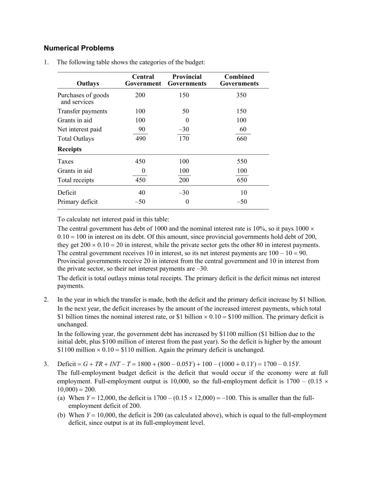
1. The following table shows the categories of the budget:
Outlays
Purchases of goods
and services
Transfer payments
Grants in aid
Net interest paid
Total Outlays
Receipts
Taxes
Grants in aid
Total receipts
Deficit
Primary deficit
Central
Government
200
Provincial
Governments
150
450
0
450
40
–50
100
100
90
490
100
100
200
–30
0
50
0
–30
170
Combined
Governments
350
550
100
650
10
–50
150
100
60
660
To calculate net interest paid in this table:
The central government has debt of 1000 and the nominal interest rate is 10%, so it pays 1000 
0.10  100 in interest on its debt. Of this amount, since provincial governments hold debt of 200, they get 200  0.10  20 in interest, while the private sector gets the other 80 in interest payments.
The central government receives 10 in interest, so its net interest payments are 100 – 10  90.
Provincial governments receive 20 in interest from the central government and 10 in interest from the private sector, so their net interest payments are –30.
The deficit is total outlays minus total receipts. The primary deficit is the deficit minus net interest payments.
2. In the year in which the transfer is made, both the deficit and the primary deficit increase by $1 billion.
In the next year, the deficit increases by the amount of the increased interest payments, which total
$1 billion times the nominal interest rate, or $1 billion  0.10  $100 million. The primary deficit is unchanged.
In the following year, the government debt has increased by $1100 million ($1 billion due to the initial debt, plus $100 million of interest from the past year). So the deficit is higher by the amount
$1100 million  0.10  $110 million. Again the primary deficit is unchanged.
3. Deficit  G  TR  INT – T  1800  (800 – 0.05
Y )  100 – (1000  0.1
Y )  1700 – 0.15
Y .
The full-employment budget deficit is the deficit that would occur if the economy were at full employment. Full-employment output is 10,000, so the full-employment deficit is 1700 – (0.15

10,000)

200.
(a) When Y  12,000, the deficit is 1700 – (0.15  12,000)  –100. This is smaller than the fullemployment deficit of 200.
(b) When Y  10,000, the deficit is 200 (as calculated above), which is equal to the full-employment deficit, since output is at its full-employment level.

(c) When Y  8000, the deficit is 1700 – (0.15  8000)  500. This is larger than the fullemployment deficit of 200.
In general, the full-employment deficit is unaffected by the state of the economy, while the actual deficit rises relative to the full-employment deficit in recessions and falls relative to the full-employment deficit in expansions.
4. (a) In this situation, someone earning income Y between $8000 and $20,000 pays a total tax of T  .25
( Y – $8000), while someone earning between $20,000 and $30,000 pays tax of T  $3000  .30
( Y – $20,000).
Someone with income of $16,000 then pays tax of .25($16,000 – $8000)  $2000. This gives an average tax rate of $2000/$16,000  12.5%, while the marginal tax rate is 25%.
Someone with income of $30,000 then pays tax of $3000  .30($30,000 – $20,000)  $6000.
This gives an average tax rate of $6000/$30,000  20%, while the marginal tax rate is 30%.
(b) In this situation, someone earning income Y between $6000 and $20,000 pays a total tax of T  .20
( Y – $6000), while someone earning between $20,000 and $30,000 pays tax of T  $2800  .30
( Y – $20,000).
Someone with income of $16,000 then pays tax of .20($16,000 – $6000)  $2000. This gives an average tax rate of $2000/$16,000  12.5%, while the marginal tax rate is 20%.
Someone with income of $30,000 then pays tax of $2800  .30($30,000 – $20,000)  $5800.
This gives an average tax rate of $5800/$30,000  19.33%, while the marginal tax rate is 30%.
(c) The person making $16,000 has the same average tax rate, but a lower marginal tax rate, so there’s no income effect, just a substitution effect toward increased labor supply. The person making $30,000 faces the same marginal tax rate, so there’s no substitution effect, but has a lower average tax rate, so the income effect tends to reduce labor supply.
5. If workers value their leisure at 90 goods per day, then 90 goods per day must be the equilibrium value of the after-tax real wage.
(a) Setting the real wage equal to the marginal product of labor gives 90  250 – N , or N  160.
Output is Y  250 N – 0.5
N 2  (250  160) – (0.5  160 2 )  27,200.
(b) With a marginal tax rate on wages of 25%, the after-tax real wage now must equal 0.75  MPN, that is, w  0.75  MPN , so 90  0.75  (250 – N ), which has the solution N  130. Output is Y 
(250  130) – (0.5  130 2 )  24,050. The cost of the distortion in terms of lost output is 27,200 –
24,050  3150.
(c) With a marginal tax rate on wages of 50%, the after-tax real wage now must equal 0.50  MPN, that is, w  0.50  MPN , so 90  0.50  (250 – N ), which has the solution N  70. Output is Y 
(250  70) – (0.5  70 2 )  15,050. The cost of the distortion in terms of lost output is 27,200 –
15,050  12,150, for changing the tax rate from 0% to 50%. Doubling the tax rate from 25% to
50% makes the distortion nearly four times as big. This suggests that taxes should be smoothed over time, since high tax rates increase the distortion more than proportionately.
6. (a) To find the largest nominal deficit that the government can run without raising the debt-GDP ratio, use Eq. (15.4) and set the change in the debt-GDP ratio equal to zero. The equation is:
Change in debt–GDP ratio  deficit/nominal GDP – [(total debt/nominal GDP) × growth rate of nominal GDP]. Plugging in the values of the known variables and setting the change in the debt-
GDP ratio equal to zero gives: 0  (deficit/nominal GDP) – [(1000/nominal GDP) × 0.10].
Multiplying both sides of the equation by nominal GDP eliminates that term from the equation, leaving 0  deficit – 100. This has the solution: deficit  100.

(b) Since the debt-GDP ratio is initially 0.6, and nominal GDP is initially 10,000, then debt must initially be 6,000. If real GDP is initially 5,000 and remains constant, then with inflation of 5%, nominal GDP must increase 5% to 10,500. The equation is: Change in debt–GDP ratio  deficit/nominal GDP – [(total debt/nominal GDP) × growth rate of nominal GDP]. Plugging in the values of the known variables and setting the change in the debt-GDP ratio equal to zero gives:
0  (deficit/10,000) – [(6,000/10,000) × 0.05], so deficit  300.
7. (a) The debt-GDP ratio is .10 at the start. After n years it is .10(1.07/1.05) n . After one year it is .102, after two years it is .104, after five years it is .110, and after ten years it is .121.
If after n years the debt-GDP ratio is 10, we want to find n such that .10(1.07/1.05) n  10. Taking logarithms of both sides of this equation and solving shows that the debt-GDP ratio exceeds 10 after 245 years. So the government must run a primary surplus at some point, as the public won’t continue to buy government bonds forever.
(b) Now, after n years the debt-GDP ratio is .10(1.07/1.08) n . After one year it is .099, after two years it is .098, after five years it is .095, and after ten years it is .091. The debt-GDP ratio is declining over time, so it will never exceed 10, and the government can roll over its debt forever. The crucial difference from part (a) is that here the growth rate of GDP exceeds the interest rate.
8. L  0.2
Y – 500 i  0.2
Y – 500 r – 500  . With Y  1000, L  200 – 500 r – 500  .
(a) When r  0.04, equating real money supply to money demand gives: M / P  L  200 – (500 
0.04) – 500   180 – 500  . Real seignorage revenue R   M / P  180  – 500  2 . The following table shows seignorage revenue ( R ) for inflation rates between 0 and 0.30. These values are plotted in Figure 15.3.
Figure 15.3

0.00
0.02
0.04
0.06
0.08
0.10
R
0.0
3.4
6.4
9.0
11.2
13.0

0.12
0.14
0.16
0.18
0.20
R
14.4
15.4
16.0
16.2
16.0

0.22
0.24
0.26
0.28
0.30
R
15.4
14.4
13.0
11.2
9.0

(b) Seignorage is maximized at   0.18.
(c) The maximum amount of seignorage revenue is 16.2.
(d) When r  0.08, equating real money supply to money demand gives: M / P  L  200 – (500 
0.08) – 500   160 – 500  . Real seignorage revenue R   M / P  160  – 500  2 . The following table shows seignorage revenue ( R ) for inflation rates between 0 and 0.30. These values are plotted in Figure 15.4.
Figure 15.4
 R  R  R
0.00
0.02
0.04
0.06
0.0
3.0
5.6
7.8
0.12
0.14
0.16
12.0
12.6
12.8
0.22 11.0
0.24
0.26
9.6
7.8
0.08 9.6 0.18 12.6 0.28 5.6
0.10 11.0 0.20 12.0 0.30 3.0
The maximum seignorage of 12.8 is attained when   0.16.
9. (a) The monetary base is growing at a 10% rate, so it increases by 0.01  $250  $25. The nominal value of seignorage over the year is $25.
(b) Deposit holders pay the inflation tax on their non-interest-bearing deposits of $600  0.10  $60.
This amount is received by banks. Banks pay the inflation tax on their non-interest-bearing reserves of $50  0.10  $5. Currency holders pay the inflation tax on their non-interest-bearing currency of $200  0.10  $20.
Overall, deposit holders pay an inflation tax of $60, banks pay an inflation tax of –$60  $5  –
$55, and currency holders pay an inflation tax of $20. The total inflation tax is $60 – $55 
$20  $25.
(c) If deposit holders get the market rate of interest on their accounts, and the market rate of interest rises with inflation, then deposit holders pay no inflation tax to banks. In this case the inflation tax is borne entirely by banks ($5) and currency holders ($20).