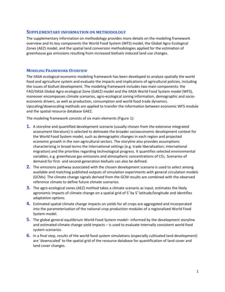
SUPPLEMENTARY INFORMATION ON METHODOLOGY
The supplementary information on methodology provides more details on the modeling framework
overview and its key components the World Food System (WFS) model, the Global Agro-Ecological
Zones (AEZ) model, and the spatial land conversion methodologies applied for the estimation of
greenhouse gas emissions resulting from increased biofuels induced land use changes.
MODELING FRAMEWORK OVERVIEW
The IIASA ecological-economic modeling framework has been developed to analyze spatially the world
food and agriculture system and evaluate the impacts and implications of agricultural policies, including
the issues of biofuel development. The modeling framework includes two main components: the
FAO/IIASA Global Agro-ecological Zone (GAEZ) model and the IIASA World Food System model (WFS),
moreover encompasses climate scenarios, agro-ecological zoning information, demographic and socioeconomic drivers, as well as production, consumption and world food trade dynamics.
Upscaling/downscaling methods are applied to transfer the information between economic WFS module
and the spatial resource database GAEZ.
The modeling framework consists of six main elements (Figure 1):
1.
2.
3.
4.
5.
6.
A storyline and quantified development scenario (usually chosen from the extensive integrated
assessment literature) is selected to delineate the broader socioeconomic development context for
the World Food System model, such as demographic changes in each region and projected
economic growth in the non-agricultural sectors. The storyline also provides assumptions
characterizing in broad terms the international settings (e.g. trade liberalization; international
migration) and the priorities regarding technological progress. It quantifies selected environmental
variables, e.g. greenhouse gas emissions and atmospheric concentrations of CO2. Scenarios of
demand for first- and second-generation biofuels can also be defined.
The emissions pathway associated with the chosen development scenario is used to select among
available and matching published outputs of simulation experiments with general circulation models
(GCMs). The climate change signals derived from the GCM results are combined with the observed
reference climate to define future climate scenarios.
The agro-ecological zones (AEZ) method takes a climate scenario as input, estimates the likely
agronomic impacts of climate change on a spatial grid of 5′ by 5′ latitude/longitude and identifies
adaptation options.
Estimated spatial climate change impacts on yields for all crops are aggregated and incorporated
into the parameterization of the national crop production modules of a regionalized World Food
System model.
The global general equilibrium World Food System model– informed by the development storyline
and estimated climate change yield impacts – is used to evaluate internally consistent world food
system scenarios.
In a final step, results of the world food system simulations (especially cultivated land development)
are ‘downscaled’ to the spatial grid of the resource database for quantification of land cover and
land cover changes.
1
Agro-ecological suitability and land productivity
3
2
Climate impact
response relations
Climate
model
1 Development
4
Production
Demand
Trade
Global
Food-FeedBiofuel System
scenario
World Market
5
6
Spatial distribution of land use
Figure 1. Ecological-economic modeling framework
World Food System (WFS) model
The World Food System model provides a framework for analyzing—in annual steps—how much food
will be produced and consumed in the world, where it will be produced and consumed, and the trade
and financial flows related to such activities. It is used to simulate alternative development scenarios, to
investigate climate change impacts on food provision, and to assess the implications of alternative
biofuel targets. It provides a framework for analyzing the world food system, viewing national food and
agricultural components as embedded in national economies, which in turn interact with each other at
the international trade level.
For current applications, a state-of-the-art ecological-economic modeling framework is used that
includes as three major components: the Global Agro-ecological Zone (GAEZ) model, the WFS model,
and upscaling/downscaling methods to transfer information between these modules and the spatial
resource database. The modeling framework and models have been developed to analyze spatially the
world food and agriculture system, its impacts on food security and the environment and to evaluate
the impacts and implications of agricultural policies.
IIASA released a first version of the WFS model in 1988, termed the Basic Linked System, in response to
the energy and food crisis of the1980s. The WFS model and its databases have been updated and
2
extended on several occasions. 1,2,3,4,5,6,7 The model has been calibrated and validated over past time
windows.
Methodology / Data generation
The WFS is a global recursive dynamic applied general equilibrium model made up of 34 national and/or
regional geographical components. The individual national/regional models are linked together by
means of a world market, where international clearing prices are computed to equalize global demand
with supply. The model is formulated as a recursively dynamic system, working in annual steps, the
outcome of each step being affected by the outcomes of earlier ones. Each individual model covers the
whole economy of the respective geographical area. For the purpose of international linkage,
production, consumption, and trade are aggregated to nine agricultural sectors and one non-agricultural
sector. All physical and financial accounts are balanced and mutually consistent: the production,
consumption, and financial ones at the national level, and the trade and financial flows at the global
level (Figure 2).
COUNTRY A
EXCHANGE
EQUILIBRIUM
PRODUCTION
Non-agriculture
production
Prices, consumption, stocks, net
exports to satisfy:
Agriculture
production
Production inputs:
• Budget constraint
• Market clearance
• Trade balance
• Trade quota
• Land
• Labour
• Capital
• Fertilizer
• Others
GOVERNMENT POLICIES
Target price, tariffs, taxes, quota, etc.
International commodity prices PW
Net trade EA
COUNTRY B
PW
WORLD MARKETS
International prices
to satisfy:
• commodity balances
• financial transfer balance
EC
PW
COUNTRY C
ED
EB
EE
PW
COUNTRY D
PW
COUNTRY E
Figure 2. Schematic representation of the World Food System model
3
The world food system model is an applied general equilibrium (AGE) model system. While focusing on
agriculture, this necessitates that also all other economic activities are represented in the model.
Financial flows as well as commodity flows within a country and at the international level are kept
consistent, in the sense that they must balance, by imposing a system of budget constraints and marketclearing conditions. Whatever is produced will be demanded, either for human consumption, feed,
biofuel use, or as intermediate input. Alternatively, commodities can be exported or put into storage.
Consistency of financial flows is imposed at the level of the economic agents in the model (individual
income groups, governments, etc.), at the national as well as the international level. This implies that
total expenditures cannot exceed total income from economic activities and from abroad, in the form of
financial transfers, minus savings. On a global scale, not more can be spent than what is earned.
Each individual model component focuses primarily on the agricultural sector, but includes also a simple
representation of the entire economy as necessary to capture essential dynamics among capital, labor
and land. For the purpose of international linkage, production, consumption and trade of goods and
services are aggregated into nine main agricultural sectors, namely: wheat; rice; coarse grains; bovine
and ovine meat; dairy products; other meat and fish; oilseed cakes and protein meals; other food; nonfood agriculture. The rest of the economy is coarsely aggregated into one simplified non-agricultural
sector. Agricultural commodities may be used in the model for human consumption, feed, as biofuel
feedstock, for intermediate consumption, and stock accumulation. The non-agricultural commodity
contributes also as investment, and as input for processing and transporting agricultural goods. All
physical and financial accounts are balanced and mutually consistent: the production, consumption, and
financial ones at the national level, and the trade and financial flows at the global level.
Linkage of country and country-group models occurs through trade, world market prices, and financial
flows. The system is solved in annual increments, simultaneously for all countries in each time period.
Within each one-year time period, demand changes with price and commodity buffer stocks can be
adjusted for short-term supply response. Production in the following marketing year (due to time lags in
the agricultural production cycle) is affected by changes in relative prices. This feature makes the world
food model a recursively dynamic system.
The market clearing process results in equilibrium prices, i.e., a vector of international prices such that
global imports and exports balance for all commodities. These market-clearing prices are then used to
determine value added in production and income of households and governments.
Within each regional unit, the supply modules allocate land, labor and capital as a function of the
relative profitability of the different crop and livestock sectors. In particular, actual cultivated acreage is
computed from both agro-climatic land parameters (derived from GAEZ) and profitability estimates.
Once acreage, labor and capital are assigned to cropping and livestock activities, yields and livestock
production is computed as a function of fertilizer applications, feed rates, and available technology.
Simulations with the WFS generate a variety of outputs for model variables and indicators. At the global
level these include world market prices, global population, global production and consumption, and
global income. At the country level the information varies with the type of model, including in general
the following variables: producer and retail prices, level of production, use of primary production factors
(land, labor, and capital), intermediate input use (feed, fertilizer, and other chemicals), human
consumption, stock levels and commodity trade, gross domestic product and investment by sector,
levels of taxes, tariffs, and income by group and/or sector.
4
GLOBAL AGRO-ECOLOGICAL ZONES (GAEZ) MODEL OVERVIEW
The AEZ approach is a GIS-based modeling framework that combines land evaluation methods with
socioeconomic and multi-criteria analysis to evaluate spatial and dynamic aspects of agriculture. The
International Institute for Applied Systems Analysis (IIASA) and the Food and Agriculture Organization of
the United Nations (FAO) have been continuously developing the Agro-Ecological Zones (AEZ)
methodology over the past 30 years for assessing agricultural resources and potential. The AEZ approach
became global in 2000 with the availability of digital global databases of climatic parameters,
topography, soil and terrain, land cover, and population distribution.
GAEZ v3.08 provides the most ambitious assessment yet, and the entire database and all results of this
assessment are available through the GAEZ Data Portal, which will be publically accessible from the
IIASA and FAO Web sites. GAEZ results are provided as a global gridded data set of 5 arc-minutes
resolution.
The GAEZ methodology uses a land resources inventory to assess, for specified management conditions
and levels of inputs, all feasible agricultural land-use options and to quantify anticipated production of
cropping activities relevant in the specific agro-ecological context. The GAEZ methodology follows an
environmental approach. It provides a standardized framework for the characterization of climate, soil,
and terrain conditions for analyzing synergies and trade-offs of alternative uses of agro-resources (land,
water, technology) for food and energy production, while preserving environmental quality. Examples of
GAEZ applications are:




Quantification of land productivity;
Estimations of rain-fed or irrigated cultivation potential for food, feed, fiber, and bio-energy
feedstock production;
Identification of environmental constraints to agricultural production; and
Identification of potential hot spots of agricultural conversion and possible geographical shifts in
agricultural land potentials due to changing climate.
Overall GAEZ model structure and data integration
There are five main steps involved in calculation procedures for establishing crop suitability estimates
(Figure 3): 1) climate data analysis and compilation of general agro-climatic indicators; 2) crop-specific
agro-climatic assessment and water-limited biomass/yield calculation; 3) assessments of yield reduction
due to agro-climatic constraints; 4) implementation of edaphic assessments to calculate yield reduction
due to soil and terrain limitations; and 5) integration of results into crop-specific grid-cell databases.
Two main activities are involved in obtaining the grid-cell level area, yield, and production of the main
crops: Estimation of shares of rain-fed or irrigated cultivated land by grid cell; and estimation of the
area, yield, and production of the main crops in rain-fed and irrigated cultivated land. Global inventories
of yield gaps were created by comparing potential rain-fed yields with yields of downscaled statistical
production.
Details of the methodology are described elsewhere. 8,9
5
Land utilization
types
Climate
resources
Spatial data sets
soil and terrain resources, land cover, protected areas,
irrigated areas, population density, livestock density,
distance to market.
Module I
Climatic
crop yields
crop constraints
crop calendars
Agro-climatic
data analysis
Land
resources
Module II
Biomass and yield
Crop statistics
Module III
Agro-climatic
attainable
yields
Agro-climatic
constraints
Module IV
Agro-edaphic
constraints
Module V
Module VI
Current crop
production
Harvested area
crop yield and
production
Crop
potentials
Suitable areas
and potential
crop yields
Module VII
Yield and production
gaps
Crop yield and
production gaps
Figure 3. Overall model structure and data integration of GAEZ v3.0 (Module I-VII)
SPATIAL LAND CONVERSIONS AS BASIS FOR GREENHOUSE GAS EMISSIONS ACCOUNTING
Land conversion in the integrated assessment framework (Figure 1) is explicitly modeled to maintain full
consistency between the spatial agro-ecological zones approach used for appraising land resources and
land productivity and the expansion of cultivated land as determined in the world food system model.
The conversion of agricultural land is allocated to the spatial grid in 10-year time steps by solving a series
of multi-criteria optimization problems for each of the countries/regions of the world food system
model.
The modeling framework (i) characterizes spatial land productivity and its current uses, (ii) uses land
cover interpretations for the base year 2000 together with statistical data from the FAO to construct
comprehensive spatial land accounts in terms of area shares for seven main land use/land cover classes,
(iii) informs the world food system model of physical resource availability and characteristics, and (iv)
updates in regular time steps the spatial resource data base and estimated spatial use consistent with
the aggregate outcomes of the world food system model.
The inventory of major land cover/land use categories has been compiled using an iterative calculation
procedure to estimate land cover class weights, consistent with aggregate FAO land statistics and spatial
land cover patterns obtained from remotely sensed data and geographic datasets, including GLC2000
land cover database, an IFPRI global land cover categorization data set, FAO's Global Forest Resources
Assessment, the Global Map of Irrigated Areas (GMIA) of FAO/University of Frankfurt, and a population
6
density inventory developed by FAO-SDRN. The results provide shares of major land use and land cover
categories within individual 5 arc-minute grid-cells. These categories are: (i) Rain-fed cultivated land; (ii)
irrigated cultivated land; (iii) forest land; (iv) grassland and woodland; (v) barren and sparsely vegetated
land; (vi) urban and other land required for housing and infrastructure, and (vii) inland water bodies.
The criteria used in the land conversion module depend on whether there is a projected net decrease or
increase of cultivated land in the region of consideration. In the case of a decrease the main criteria and
drivers include demand for built-up land and abandonment of marginally productive cultivated land. In
case of increases of cultivated land the land conversion algorithm takes land demand from the world
food system equilibrium and applies several constraints and criteria, including: (i) the total amount of
land converted from and to agriculture in each region of the world food system model, (ii) the
productivity, availability and current use of land resources in each country/region of the world food
system model, (iii) suitability of land for conversion to crop production, (iv) legal land use limitation, i.e.
protection status, (v) spatial suitability/propensity of ecosystems to be converted to agricultural land,
i.e. a priority ranking of ecosystems with regard to land conversion, and (vi) land accessibility, i.e. in
particular a grid-cell’s distance from existing crop production activities.
To ensure comparability across scenarios the above criteria, rules and parameterization guiding land
conversion have been kept the same for all scenario simulations in this study.
A carbon accounting method, based on IPCC Tier 1 approaches10, is used to quantify for each scenario
changes of vegetation and soil carbon pools.
References
1. Fischer G., K. Frohberg, M.A. Keyzer, K.S. Parikh. Linked National Models: a Tool for International
Policy Analysis, 1988. Kluwer Academic Publishers, 214pp.
2. Parikh K.S., Fischer G., Frohberg K., Gulbrandsen O. 1988. Towards free trade in agriculture.
International Institute for Applied Systems Analysis. ISBN 90-247-3632-3. Martinus Nijhoff Publishers.
3. Fischer, G., Frohberg, K., Parry, M.L., and Rosenzweig, C. (1994). Climate Change and World Food
Supply, Demand and Trade: Who Benefits, Who Loses? Global Environmental Change 4(1), 7–23.
4. Fischer, G., M. Shah and H. van Velthuizen (2002). Climate Change and Agricultural Vulnerability.
Special Report as contribution to the World Summit on Sustainable Development, Johannesburg 2002.
International Institute for Applied Systems Analysis, Laxenburg, Austria. pp 152.
5. Fischer, G., M. Shah, F.N. Tubiello, H van Velhuizen (2005). Socio-economic and climate change
impacts on agriculture: an integrated assessment, 1990–2080. Phil. Trans. Royal Soc. B,
doi:10.1098/rstb.2005.1744.
6. Fischer, G., E. Hizsnyik, S. Prieler, M. Shah, and H. van Velthuizen (2009). Biofuels and Food Security.
The OPEC Fund for International Development (OFID) and International Institute of Applied Systems
Analysis (IIASA), Vienna, Austria, 228 pp.
7. Fischer G. and Prieler S.. Impacts of biofuel expansion on world food systems and the environment. A
global agricultural ecological-economic modelling framework for scenario analysis. ELOBIO Deliverable
5.2 and 5.3. Intelligent Energy Europe. 2010. 66 pp.
http://www.elobio.eu/fileadmin/elobio/user/docs/D5.2_5.3.pdf
7
8. Fischer, G., Nachtergaele, F., Prieler, S., Teixeira, E., Tóth, G., van Velthuizen, H., Verelst, L., Wiberg,
D.: GAEZ v3.0 Global Agro-Ecological Zones - Model Documentation. International Institute for Applied
systems Analysis (IIASA), Laxenburg, Austria and the Food and Agriculture Organization of the United
Nations (FAO) Rome, Italy. 2012. Available at:
http://typo3.fao.org/fileadmin/user_upload/gaez/docs/GAEZ_Model_Documentation.pdf
9. Fischer G., van Velthuizen H., Shah M, Nachtergaele F.O. Global Agro-ecological Assessment for
Agriculture in the 21st Century. Methodology and Results. IIASA RR-02-02. IIASA, 2002. Laxenburg,
Austria. http://www.iiasa.ac.at/Admin/PUB/Documents/RR-02-002.pdf
10. Penman, J., Gytarsky, M., Hiraishi, T., Krug, T., Kruger, D., Pipatti, R., Buendia, L., Miwa, K., Ngara, T.,
Tanabe, K., Wagner, F., 2003. Good Practice Guidance for Land Use, Land-Use Change and Forestry. IPCC
National Greenhouse Gas Inventories Programme and Institute for Global Environmental Strategies,
Kanagawa, Japan. http://www.ipcc-nggip.iges.or.jp/public/gpglulucf/gpglulucf.html
8