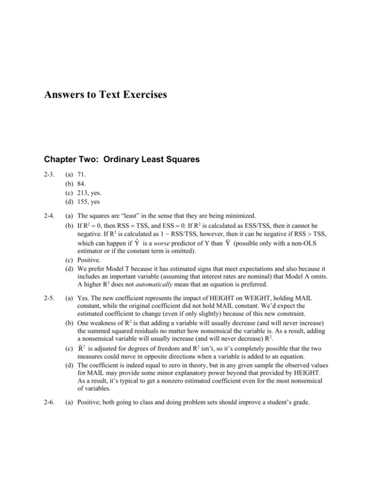
Answers to Text Exercises
Chapter Two: Ordinary Least Squares
2-3.
(a)
(b)
(c)
(d)
71.
84.
213, yes.
155, yes
2-4.
(a) The squares are “least” in the sense that they are being minimized.
(b) If R2  0, then RSS  TSS, and ESS  0. If R2 is calculated as ESS/TSS, then it cannot be
negative. If R2 is calculated as 1  RSS/TSS, however, then it can be negative if RSS  TSS,
which can happen if Ŷ is a worse predictor of Y than Y (possible only with a non-OLS
estimator or if the constant term is omitted).
(c) Positive.
(d) We prefer Model T because it has estimated signs that meet expectations and also because it
includes an important variable (assuming that interest rates are nominal) that Model A omits.
A higher R2 does not automatically mean that an equation is preferred.
2-5.
(a) Yes. The new coefficient represents the impact of HEIGHT on WEIGHT, holding MAIL
constant, while the original coefficient did not hold MAIL constant. We’d expect the
estimated coefficient to change (even if only slightly) because of this new constraint.
(b) One weakness of R2 is that adding a variable will usually decrease (and will never increase)
the summed squared residuals no matter how nonsensical the variable is. As a result, adding
a nonsensical variable will usually increase (and will never decrease) R2.
(c) R2 is adjusted for degrees of freedom and R2 isn’t, so it’s completely possible that the two
measures could move in opposite directions when a variable is added to an equation.
(d) The coefficient is indeed equal to zero in theory, but in any given sample the observed values
for MAIL may provide some minor explanatory power beyond that provided by HEIGHT.
As a result, it’s typical to get a nonzero estimated coefficient even for the most nonsensical
of variables.
2-6.
(a) Positive; both going to class and doing problem sets should improve a student’s grade.
(b) Yes.
(c) 0.04  1.74  0.02  0.60, so going to class pays off more.
(d) 0.02  1.74  0.10  0.60, so doing problem sets pays off more. Since the units of variables
can differ dramatically, coefficient size does not measure importance. (If all variables are
measured identically in a properly specified equation, then the size of the coefficient is indeed
one measure of importance.)
(e) An R2 of 0.33 means that a third of the variation of student grades around their mean can be
explained by attendance at lectures and the completion of problem sets. This might seem low
to many beginning econometricians, but in fact it’s either about right or perhaps even a bit
higher than we might have expected.
(f) The most likely variable to add to this equation is the ith student’s GPA or some other
measure of student ability. We’d expect both R2 and R2 to rise.
2-7.
(a) Even though the fit in Equation A is better, most researchers would prefer Equation B
because the signs of the estimated coefficients are as would be expected. In addition, X4 is a
theoretically sound variable for a campus track, while X3 seems poorly specified because an
especially hot or cold day would discourage fitness runners.
(b) The coefficient of an independent variable tells us the impact of a one-unit increase in that
variable on the dependent variable holding constant the other explanatory variables in the
equation. If we change the other variables in the equation, we’re holding different variables
constant, and so the ̂ has a different meaning.
2-8.
(a)
(b)
(c)
(d)
2-9.
As we’ll learn in Chapters 6 and 7, there’s a lot more to specifying an equation than
maximizing R 2 .
2-10.
(a) Vi: positive.
Hi: negative (although some would argue that in a world of perfect information, drivers
would take fewer risks if they knew the state had few hospitals).
Ci: ambiguous because a high rate of driving citations could indicate risky driving (raising
fatalities) or zealous police citation policies (reducing risky driving and therefore fatalities).
(b) No, because the coefficient differences are small and the data will differ from year to year.
We’d be more concerned if the coefficients differed by orders of magnitude or changed sign.
(c) Since the equation for the second year has similar degrees of freedom and a much lower R2,
no calculation is needed to know that the equation for the first year has a higher R2. Just to be
sure, we calculated R2 and obtained 0.652 for the first year and 0.565 for the second year.
2-11.
(a) It might seem that the higher the percentage body fat, the higher the weight, holding constant
height, but muscle weighs more than fat, so it’s possible that a lean, highly muscled man
could weigh more than a less well-conditioned man of the same height.
(b) We prefer Equation 1.24 because we don’t think F belongs in the equation on theoretical
grounds. The meaning of the coefficient of X changes in that F now is held constant.
(c) The fact that R2 drops when the percentage body fat is introduced to the equation strengthens
our preference for Equation 1.24.
(d) This is subtle, but since 0.28 times 12.0 equals 3.36, we have reason to believe that the
impact of bodyfat on weight (holding constant height) is very small indeed. That is, moving
from average bodyfat to no bodyfat would lower your weight by only 3.36 pounds.
Yes.
At first glance, perhaps, but see below.
Three dissertations, since (978  3)  $2934 > (204  2  36  2)  $480  ($460  1)  $460
The coefficient of D seems to be too high; perhaps it is absorbing the impact of an
independent variable that has been omitted from the regression. For example, students may
choose a dissertation adviser on the basis of reputation, a variable not in the equation.
2-12.
(a) (e2i )/ˆ  2(Yi  ˆ0  ˆ1X i )(1)
(e2i )/ˆ1  2(Yi  ˆ0  ˆ1X i )( ˆ1X i )
(b) 0  2(Yi  ˆ0  ˆ1Xi )
0  2 ˆ1(Yi  ˆ0  ˆ1Xi )(Xi ) or, rearranging:
Yi  nˆ0  ˆ1X i
Y X ˆ X  ˆ X2
i
i
0
i
1
i
These are the normal equations.
(c) To get ˆ1 , solve the first normal equation for ˆ0 , obtaining
ˆ  (Y   X )/N and substitute this value in for ˆ where it appears in
0
i
1
i
0
the second normal equation, obtaining Yi Xi  (Yi  ˆ1Xi )(Xi )/N  ˆ1X2i , which
becomes ˆ  (NY X  Y X ) /[NX2  (X )2 ]. With some algebraic manipulation
1
i
i
i
i
i
i
(in part using the fact that Xi  NX), this simplifies to Equation 2.4.
(d) To get Equation 2.5, solve the first normal equation for ˆ0 , using X  Xi /N.
2-13.
(a) Yes. We’d expect bigger colleges to get more applicants, and we’d expect colleges that used
the common application to attract more applicants. It might seem at first that the rank of a
college ought to have a positive coefficient, but the variable is defined as 1  best, so we’d
expect a negative coefficient for RANK.
(b) The meaning of the coefficient of SIZE is that for every increase of one in the size of the
student body, we’d expect a college to generate 2.15 more applications, holding RANK and
COMMONAP constant. The meaning of the coefficient of RANK is that every one-rank
improvement in a college’s U.S. News ranking should generate 32.1 more applications,
holding SIZE and COMMONAP constant. These results do not allow us to conclude that a
college’s ranking is 15 times more important than the size of that college because the units of
the variables SIZE and RANK are quite different in magnitude. On a more philosophical
level, it’s risky to draw any general conclusions at all from one regression estimated on a
sample of 49 colleges.
(c) The meaning of the coefficient of COMMONAP is that a college that switches to using the
common application can expect to generate 1222 more applications, holding constant RANK
and SIZE. However, this result does not prove that a given college would increase
applications by 1222 by switching to the common application. Why not? First, we don’t trust
this result because there may well be an omitted relevant variable (or two) and because all but
three of the colleges in the sample use the common application. Second, in general,
econometric results are evidence that can be used to support an argument, but in and of
themselves they don’t come close to “proving” anything.
(e) If you drop COMMONAP from the equation, R2 falls from 0.681. This is evidence (but not
proof) that COMMONAP belongs in the equation.