Lesson 10
NYS COMMON CORE MATHEMATICS CURRICULUM
6•6
Lesson 10: Describing Distributions Using the Mean and
MAD
Student Outcomes

Students calculate the mean and MAD for a data distribution.

Students use the mean and MAD to describe a data distribution in terms of center and variability.
Classwork
Example 1 (8 minutes): Describing Distributions
Example 1: Describing Distributions
In Lesson 9, Sabina developed the mean absolute deviation (MAD) as a number that measures variability in a data
distribution. Using the mean and MAD with a dot plot allows you to describe the center, spread, and shape of a data
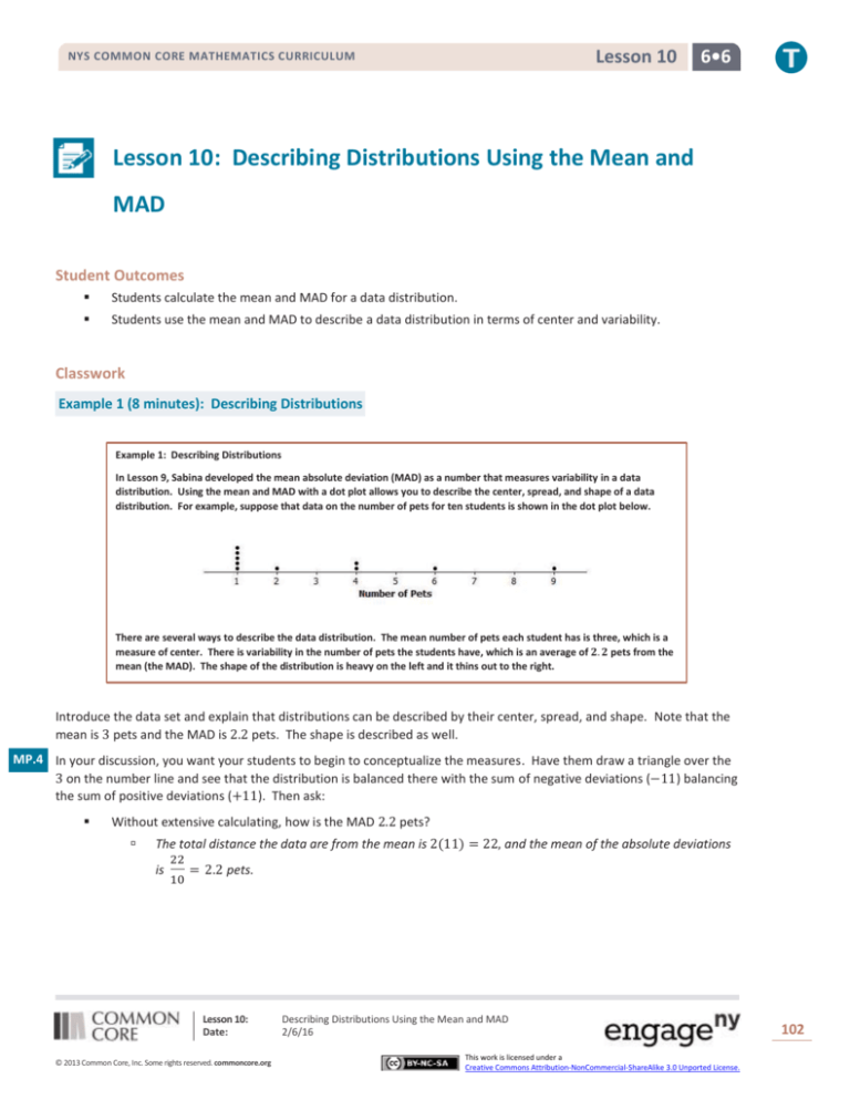
distribution. For example, suppose that data on the number of pets for ten students is shown in the dot plot below.
There are several ways to describe the data distribution. The mean number of pets each student has is three, which is a
measure of center. There is variability in the number of pets the students have, which is an average of 𝟐. 𝟐 pets from the
mean (the MAD). The shape of the distribution is heavy on the left and it thins out to the right.
Introduce the data set and explain that distributions can be described by their center, spread, and shape. Note that the
mean is 3 pets and the MAD is 2.2 pets. The shape is described as well.
MP.4 In your discussion, you want your students to begin to conceptualize the measures. Have them draw a triangle over the
3 on the number line and see that the distribution is balanced there with the sum of negative deviations (−11) balancing
the sum of positive deviations (+11). Then ask:

Without extensive calculating, how is the MAD 2.2 pets?

The total distance the data are from the mean is 2(11) = 22, and the mean of the absolute deviations
is
22
10
= 2.2 pets.
Lesson 10:
Date:
© 2013 Common Core, Inc. Some rights reserved. commoncore.org
Describing Distributions Using the Mean and MAD
2/6/16
This work is licensed under a
Creative Commons Attribution-NonCommercial-ShareAlike 3.0 Unported License.
102
Lesson 10
NYS COMMON CORE MATHEMATICS CURRICULUM
6•6
Exercises 1–4 (9–12 minutes)
Let students work with a partner. Then discuss and confirm answers to Exercises 1–3.
Exercises 1–4
1.
Suppose that the weights of seven middle-school students’ backpacks are given below.
a.
Fill in the following table.
Student
Weight (lbs.)
Deviations
Absolute
Deviations
b.
Alan
𝟏𝟖
𝟎
Beth
𝟏𝟖
𝟎
Char
𝟏𝟖
𝟎
Damon
𝟏𝟖
𝟎
Elisha
𝟏𝟖
𝟎
Fred
𝟏𝟖
𝟎
Georgia
𝟏𝟖
𝟎
𝟎
𝟎
𝟎
𝟎
𝟎
𝟎
𝟎
Draw a dot plot for these data and calculate the mean and MAD.
The mean is 𝟏𝟖 pounds.
The MAD is 𝟎.
c.
Describe this distribution of weights of backpacks by discussing the center, spread, and shape.
The mean is 𝟏𝟖 pounds. There is no variability.
All of the data is centered.
2.
Suppose that the weight of Elisha’s backpack is 𝟏𝟕 pounds, rather than 𝟏𝟖.
a.
Draw a dot plot for the new distribution.
b.
Without doing any calculation, how is the mean affected by the lighter weight? Would the new mean be the
same, smaller, or larger?
The mean will be smaller because the new point is smaller.
c.
Without doing any calculation, how is the MAD affected by the lighter weight? Would the new MAD be the
same, smaller, or larger?
Now there is variability, so the MAD is greater than zero.
Lesson 10:
Date:
© 2013 Common Core, Inc. Some rights reserved. commoncore.org
Describing Distributions Using the Mean and MAD
2/6/16
This work is licensed under a
Creative Commons Attribution-NonCommercial-ShareAlike 3.0 Unported License.
103
Lesson 10
NYS COMMON CORE MATHEMATICS CURRICULUM
3.
6•6
Suppose that in addition to Elisha’s backpack weight having changed from 𝟏𝟖 to 𝟏𝟕 lb., Fred’s backpack weight is
changed from 𝟏𝟖 to 𝟏𝟗 lb.
a.
Draw a dot plot for the new distribution.
b.
Without doing any calculation, what would be the value of the new mean compared to the original mean?
The mean is 𝟏𝟖 lbs.
c.
Without doing any calculation, would the MAD for the new distribution be the same, smaller, or larger than
the original MAD?
Since there is more variability, the MAD is larger.
d.
Without doing any calculation, how would the MAD for the new distribution compare to the one in Exercise
2?
There is more variability, so the MAD is greater than in Exercise 2.
4.
Suppose that seven second-graders’ backpack weights were:
Student
Weight (lbs.)
a.
Alice
𝟓
Bob
𝟓
Carol
𝟓
Damon
𝟓
Ed
𝟓
Felipe
𝟓
Gale
𝟓
How is the distribution of backpack weights for the second-graders similar to the original distribution for
sixth-graders given in Exercise 1?
Both have no variability, so the MAD is zero. The dot plots look the same.
b.
How are the distributions different?
The means are different. One mean is 𝟏𝟖 and the other is 𝟓.
Example 2 (5 minutes): Using the Mean Versus the MAD
Example 2: Using the Mean Versus the MAD
Decision-making by comparing distributions is an important function of statistics. Recall that Robert is trying to decide
whether to move to New York City or to San Francisco based on temperature. Comparing the center, spread, and shape
for the two temperature distributions could help him decide.
Lesson 10:
Date:
© 2013 Common Core, Inc. Some rights reserved. commoncore.org
Describing Distributions Using the Mean and MAD
2/6/16
This work is licensed under a
Creative Commons Attribution-NonCommercial-ShareAlike 3.0 Unported License.
104
Lesson 10
NYS COMMON CORE MATHEMATICS CURRICULUM
6•6
From the dot plots, Robert saw that monthly temperatures in New York City were spread fairly evenly from around 𝟒𝟎
degrees to the 𝟖𝟎s, but in San Francisco the monthly temperatures did not vary as much. He was surprised that the mean
temperature was about the same for both cities. The MAD of 𝟏𝟒 degrees for New York City told him that, on average, a
month’s temperature was 𝟏𝟒 degrees above or below 𝟔𝟑 degrees. That is a lot of variability, which was consistent with
the dot plot. On the other hand, the MAD for San Francisco told him that San Francisco’s monthly temperatures differ, on
average, only 𝟑. 𝟓 degrees from the mean of 𝟔𝟒 degrees. So, the mean doesn’t help Robert very much in making a
decision, but the MAD and dot plot are helpful.
Which city should he choose if he loves hot weather and really dislikes cold weather?
Read through the example as a class. Note that, although the mean provides useful information, it does not give an
accurate picture of the spread of monthly temperatures for New York City. It is important to consider the center,
MP.2 spread, and shape of distributions when making decisions.
Let students answer the questions:

Which city should he choose if he loves hot weather and really dislikes cold weather?


San Francisco, because there is little variability and it does not get as cold as New York city.
What measure of the data would justify your decision? Why did you choose that measure?

The mean absolute deviation (MAD) as it provides a measure of the variability. On average, the
monthly temperatures in San Francisco do not vary as much from the mean monthly temperature.
Exercises 5–7 (15–20 minutes)
Give students an opportunity to work independently. Let them confirm answers with a neighbor as needed. If time
allows, discuss answers as a class. Allow students to use calculators for this exercise. Prioritize your discussion of
questions, as Exercise 7 is the first time students see a dot plot with the same MAD and mean.
Exercises 5–7
5.
Robert wants to compare temperatures for Cities B and C.
City B
City C
a.
J
𝟓𝟒
𝟓𝟒
F
𝟓𝟒
𝟒𝟒
M
𝟓𝟖
𝟓𝟒
A
𝟔𝟑
𝟔𝟏
M
𝟔𝟑
𝟔𝟑
J
𝟔𝟖
𝟕𝟐
J
𝟕𝟐
𝟕𝟖
A
𝟕𝟐
𝟖𝟓
S
𝟕𝟐
𝟕𝟖
O
𝟔𝟑
𝟓𝟗
N
𝟔𝟑
𝟓𝟒
D
𝟓𝟒
𝟓𝟒
Draw a dot plot of the monthly temperatures for each of the cities.
Lesson 10:
Date:
© 2013 Common Core, Inc. Some rights reserved. commoncore.org
Describing Distributions Using the Mean and MAD
2/6/16
This work is licensed under a
Creative Commons Attribution-NonCommercial-ShareAlike 3.0 Unported License.
105
Lesson 10
NYS COMMON CORE MATHEMATICS CURRICULUM
b.
6•6
Verify that the mean monthly temperature for each distribution is 𝟔𝟑 degrees.
The data is nearly symmetrical around 𝟔𝟑 degrees for City B.
The sum of positive deviations is +𝟔𝟏, and the sum of the negative deviations is −𝟔𝟏 around the mean of 𝟔𝟑
for City C.
c.
Find the MAD for each of the cities. Interpret the two MADs in words and compare their values.
The MAD is 𝟓. 𝟑 degrees for City B, which means, on average, a month’s temperature differs from 𝟔𝟑 degrees
by 𝟓. 𝟑 degrees.
The MAD is 𝟏𝟎. 𝟐 for City C, which means, on average, a month’s temperature differs from 𝟔𝟑 degrees by
𝟏𝟎. 𝟐 degrees.
6.
How would you describe the differences in the shapes of the monthly temperature distributions of the two cities?
The temperatures are nearly symmetric around the mean in City B. The temperatures are compact to the left of the
mean for City C and then spread out to the right (skewed right).
7.
Suppose that Robert had to decide between Cities D, E, and F.
City D
City E
City F
J
𝟓𝟒
𝟓𝟔
𝟒𝟐
F
𝟒𝟒
𝟓𝟔
𝟒𝟐
M
𝟓𝟒
𝟓𝟔
𝟕𝟎
A
𝟓𝟗
𝟓𝟔
𝟕𝟎
M
𝟔𝟑
𝟓𝟔
𝟕𝟎
J
𝟕𝟐
𝟖𝟒
𝟕𝟎
J
𝟕𝟖
𝟖𝟒
𝟕𝟎
A
𝟖𝟕
𝟖𝟒
𝟕𝟎
S
𝟕𝟖
𝟓𝟔
𝟕𝟎
O
𝟓𝟗
𝟓𝟔
𝟕𝟎
N
𝟓𝟒
𝟓𝟔
𝟕𝟎
D
𝟓𝟒
𝟓𝟔
𝟒𝟐
a.
Draw dot plots for each distribution.
b.
Interpret the MAD for the distributions. What does this mean about variability?
Mean
𝟔𝟑
𝟔𝟑
𝟔𝟑
MAD
𝟏𝟎. 𝟓
𝟏𝟎. 𝟓
𝟏𝟎. 𝟓
The MADs are all the same, so Robert needs to look more at the shapes of the distributions to help him make
a decision.
Lesson 10:
Date:
© 2013 Common Core, Inc. Some rights reserved. commoncore.org
Describing Distributions Using the Mean and MAD
2/6/16
This work is licensed under a
Creative Commons Attribution-NonCommercial-ShareAlike 3.0 Unported License.
106
Lesson 10
NYS COMMON CORE MATHEMATICS CURRICULUM
c.
6•6
How will Robert decide to which city he should move? List possible reasons Robert might have for choosing
each city.
City D – Appears to have “four seasons” with widespread temperatures.
City E – Has mainly cold weather and is only hot for 𝟑 months.
City F – Has mainly moderate weather and only a few cold months.
Lesson Summary
A data distribution can be described in terms of its center, spread, and shape.

The center can be measured by the mean.

The spread can be measured by the mean absolute deviation (MAD).

A dot plot shows the shape of the distribution.
Exit Ticket (5 minutes)
Lesson 10:
Date:
© 2013 Common Core, Inc. Some rights reserved. commoncore.org
Describing Distributions Using the Mean and MAD
2/6/16
This work is licensed under a
Creative Commons Attribution-NonCommercial-ShareAlike 3.0 Unported License.
107
Lesson 10
NYS COMMON CORE MATHEMATICS CURRICULUM
Name ___________________________________________________
6•6
Date____________________
Lesson 10: Describing Distributions Using the Mean and MAD
Exit Ticket
1.
A dot plot of times that five students studied for a test is displayed below.
a.
Use the table to determine the mean number of hours that these five students studied. Then, complete the
table.
Student
Number of study hours
Deviations
Absolute deviations
b.
2.
Aria
1
Ben
1
Chloe
1.5
Dellan
2
0
Emma
4.5
Find and interpret the MAD for this data set.
The same five students are preparing to take a second test. Suppose that the data were the same except that Ben
studied 2.5 hours for the second test (1.5 hours more) and Emma studied only 3 hours for the second test (1.5
hours less.)
a.
Without doing any calculations, is the mean for the second test the same, higher, or lower than the mean for
the first test? Explain your reasoning.
b.
Without doing any calculations, is the MAD for the second test the same, higher, or lower than the MAD for
the first test? Explain your reasoning.
Lesson 10:
Date:
© 2013 Common Core, Inc. Some rights reserved. commoncore.org
Describing Distributions Using the Mean and MAD
2/6/16
This work is licensed under a
Creative Commons Attribution-NonCommercial-ShareAlike 3.0 Unported License.
108
Lesson 10
NYS COMMON CORE MATHEMATICS CURRICULUM
6•6
Exit Ticket Sample Solutions
1.
A dot plot of times that five students studied for a test is displayed below.
a.
Use the table to determine the mean number or hours that these five students studied. Then, complete the
table.
The mean is 𝟐 hours since the deviation around 𝟐 hours is 𝟎.
Student
Number of study hours
Deviations
Absolute deviations
b.
Aria
𝟏
−𝟏
𝟏
Ben
𝟏
−𝟏
𝟏
Chloe
𝟏. 𝟓
−𝟏. 𝟓
−𝟎. 𝟓
Dellan
𝟐
𝟎
𝟎
Emma
𝟒. 𝟓
𝟐. 𝟓
𝟐. 𝟓
Find and interpret the MAD for this data set.
The MAD is
𝟏 + 𝟏 + 𝟎.𝟓 + 𝟐.𝟓
𝟓
= 𝟏 hour.
On average the students studied 𝟏 hour away from the group mean of 𝟐 hours.
2.
The same five students are preparing to take a second test. Suppose that the data were the same, except that Ben
studied 𝟐. 𝟓 hours for the second test (𝟏. 𝟓 hours more), and that Emma studied only 𝟑 hours for the second test
(𝟏. 𝟓 hours less).
a.
Without doing any calculations, is the mean for the second test the same, higher, or lower than the mean for
the first test? Explain your reasoning.
The mean would be the same since the distance that one data point moved to the right was matched by the
distance another data point moved to the left. The distribution is balanced at the same place.
b.
Without doing any calculations, is the MAD for the second test the same, higher, or lower than the MAD for
the first test? Explain your reasoning.
The MAD would be smaller since the data points are clustered closer to the mean.
Problem Set Sample Solutions
1.
Draw a dot plot of the times that five students studied for a test if the mean time they studied was two hours and
the MAD was zero hours.
Since the MAD is 𝟎, all data points are the same and that would be the mean value.
Lesson 10:
Date:
© 2013 Common Core, Inc. Some rights reserved. commoncore.org
Describing Distributions Using the Mean and MAD
2/6/16
This work is licensed under a
Creative Commons Attribution-NonCommercial-ShareAlike 3.0 Unported License.
109
Lesson 10
NYS COMMON CORE MATHEMATICS CURRICULUM
2.
6•6
Suppose the times that five students studied for a test is as follows:
Student
Time (hrs.)
Aria
𝟏. 𝟓
Ben
𝟐
Chloe
𝟐
Dellan
𝟐. 𝟓
Emma
𝟐
Michelle said that the MAD for this data set is 𝟎 because the dot plot is balanced around 𝟐. Without doing any
calculation, do you agree with Michelle? Why or why not?
No, Michelle is wrong. There is variability within the data set, so the MAD is greater than zero.
Note: If students agree with Michelle, then they have not yet mastered that the MAD is measuring variability. They
need to grasp that if data points differ in a distribution, whether the distribution is symmetric or not, then there is
variability. Therefore, the MAD cannot be zero.
3.
Suppose that the number of text messages eight students receive on a typical day is as follows:
Student
Number
𝟏
𝟒𝟐
𝟐
𝟓𝟔
𝟑
𝟑𝟓
𝟒
𝟕𝟎
𝟓
𝟓𝟔
𝟔
𝟓𝟎
𝟕
𝟔𝟓
𝟖
𝟓𝟎
a.
Draw a dot plot for the number of text messages received on a typical day by these eight students.
b.
Find the mean number of text messages these eight students receive on a typical day.
Since the distribution appears to be somewhat symmetrical around a value in the 𝟓𝟎s, one could guess a
value for the mean, such as 𝟓𝟐 or 𝟓𝟑, and then check sums of positive and negative deviations. Using the
formula, the mean is
c.
𝟒𝟐𝟒
𝟖
= 𝟓𝟑 text messages.
Find the MAD number of text messages and explain its meaning using the words of this problem.
The sum of the positive deviations from 𝟓𝟑 is: 𝟐(𝟓𝟔 − 𝟓𝟑) + (𝟔𝟓 − 𝟓𝟑) + (𝟕𝟎 − 𝟓𝟑) = 𝟔 + 𝟏𝟐 + 𝟏𝟕 = 𝟑𝟓.
So,
𝟐(𝟑𝟓)
𝟖
yields a MAD of 𝟖. 𝟕𝟓 text messages.
This means that, on average, the number of text messages these eight students receive on a typical day is
𝟖. 𝟕𝟓 messages away from the group mean of 𝟓𝟑 messages.
d.
Describe the shape of this data distribution.
The shape of this distribution is fairly symmetrical (balanced) around the mean of 𝟓𝟑 messages.
e.
Suppose that in the original data set, Student 3 receives an additional five more text messages per day, and
Student 4 receives five fewer messages per day.
i.
Without doing any calculation, does the mean for the new data set stay the same, increase, or decrease
as compared to the original mean? Explain your reasoning.
The mean would remain at 𝟓𝟑 messages because one data point moved the same number of units to
the right as another data point moved to the left. So, the balance point of the distribution does not
change.
ii.
Without doing any calculation, does the MAD for the new data set stay the same, increase, or decrease
as compared to the original MAD? Explain your reasoning.
Since the lowest data point moved closer to the mean and the highest data point moved closer to the
mean, the variability in the resulting distribution would be more compact than the original
distribution. So, the MAD would decrease.
Lesson 10:
Date:
© 2013 Common Core, Inc. Some rights reserved. commoncore.org
Describing Distributions Using the Mean and MAD
2/6/16
This work is licensed under a
Creative Commons Attribution-NonCommercial-ShareAlike 3.0 Unported License.
110