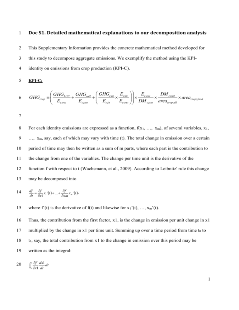
1
Doc S1. Detailed mathematical explanations to our decomposition analysis
2
This Supplementary Information provides the concrete mathematical method developed for
3
this study to decompose aggregate emissions. We exemplify the method using the KPI-
4
identity on emissions from crop production (KPI-C).
5
KPI-C:
6
 GHGLUC GHGsoil  GHGc;in Ec;in   Ec;out
DM c;out
 
GHGcrop  

 


 areacrop; food
 Ec;out
Ec;out
Ec;out   DM c;out areacrop;all
 Ec;in

7
8
For each identity emissions are expressed as a function, f(x1, …, xm), of several variables, x1,
9
…, xm, say, each of which may vary with time (t). The total change in emission over a certain
10
period of time may then be written as a sum of m parts, where each part is the contribution to
11
the change from one of the variables. The change per time unit is the derivative of the
12
function f with respect to t (Wachsmann, et al., 2009). According to Leibnitz' rule this change
13
may be decomposed into
14
df
f
f

x1 ' t   ... 
xm ' t  ,
dt x1
xm
15
where f’(t) is the derivative of f(t) and likewise for x1’(t), …, xm’(t).
16
Thus, the contribution from the first factor, x1, is the change in emission per unit change in x1
17
multiplied by the change in x1 per time unit. Summing up over a time period from time t0 to
18
t1, say, the total contribution from x1 to the change in emission over this period may be
19
written as the integral:
20

t1
t0
f dx1
dt
x1 dt
1
21
In the KPI-C the emissions from crop production are a sum of three terms, each of which is a
22
product of a number of factors. The second term, for example, may be written y=x1·x2·x3·x4,
23
where x1=GHGsoil/Ec;out, x2= Ec;out/DMc;out, x3=DMc;out/areacrop;all and x4= areacrop;food. The
24
contribution from x1 to the change from t0 to t1 may be written as (Wachsmann, et al., 2009):
25
y
t1
     ,
ln y  ln y 
 yt0  ln x1t1  ln x1t0
t1
t0
26
which is based on an interpolation of x1t by an exponential function from time t0 to time t1.
27
Exponential interpolation is possible only for variables with positive values, but the first term
28
in KPI-C has a factor, x1=GHGLUC/Ec;out, which may take negative values. For such a variable
29
we use linear interpolation and obtain its contribution, Cx1, to the change as
30
C x1 
31
when the other three variables are positive, and we have used the notation r2=ln(x2t1)-ln(x2t0)
32
for the logarithmic change in x2 and similarly for x3 and x4. In this case the contribution from
33
x2 is given by:
34
Cx2 
35
with similar expressions for Cx3 and Cx4.
36
Finally, all contributions from each specific variable are added to obtain the contribution from
37
that variable to the total change.
38
References
39
Wachsmann, U., Wood, R., Lenzen, M. & Schaeffer, R. (2009): Structural decomposition of
40
energy use in Brazil from 1970 to 1996. Applied Energy. Vol. 86:4, pp. 578-587.
x1
t1
y
t1

 x0 t0  x 2 t1  x3t1  x 4 t1  x 2 t  x3t0  x 4 t0
r 2  r 3  r 4

 yt0  C x1  r 2
(r 2  r 3  r 4)
0
,
,
2