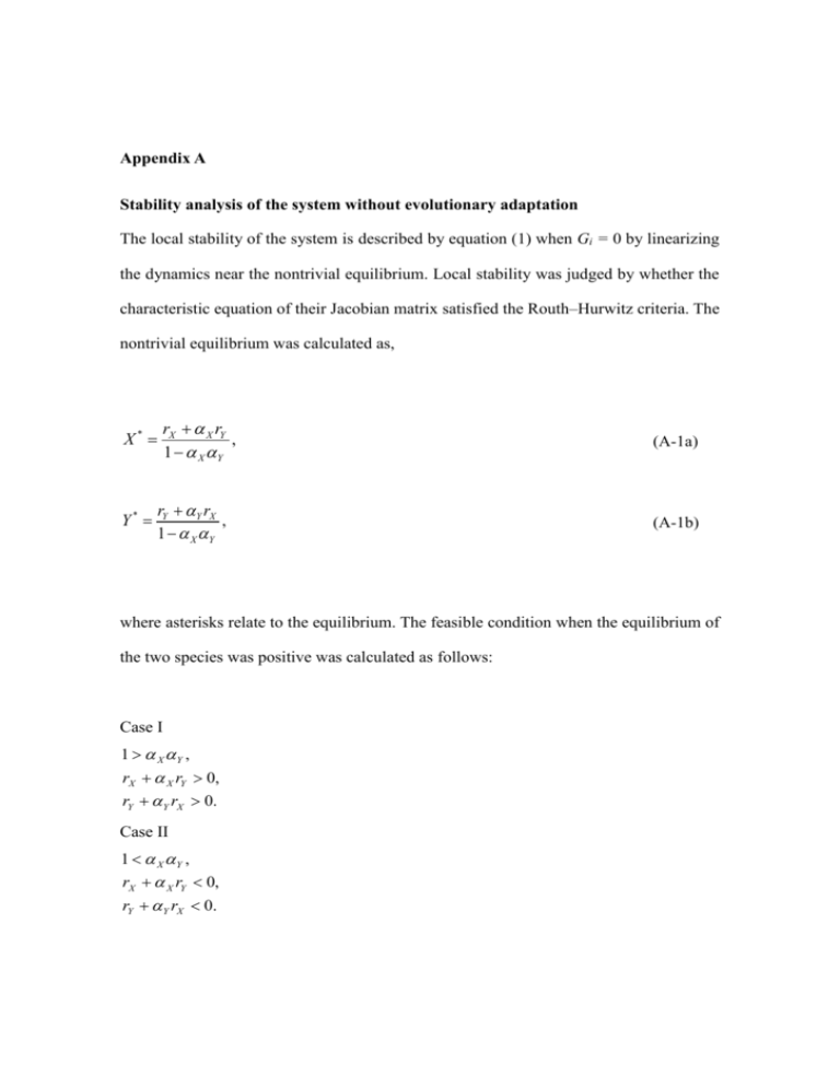
Appendix A
Stability analysis of the system without evolutionary adaptation
The local stability of the system is described by equation (1) when Gi = 0 by linearizing
the dynamics near the nontrivial equilibrium. Local stability was judged by whether the
characteristic equation of their Jacobian matrix satisfied the Routh–Hurwitz criteria. The
nontrivial equilibrium was calculated as,
X* 
Y* 
rX   X rY
,
1   X Y
rY   Y rX
,
1   X Y
(A-1a)
(A-1b)
where asterisks relate to the equilibrium. The feasible condition when the equilibrium of
the two species was positive was calculated as follows:
Case I
1   X Y ,
rX   X rY  0,
rY   Y rX  0.
Case II
1   X Y ,
rX   X rY  0,
rY   Y rX  0.
The two cases defined above correspond to facultative and obligate mutualism,
respectively.
Under the equilibrium condition, the Jacobian matrix was calculated as follows:
 r  2X *   XY *
J   X
Y Y *


X X *
.
*
*
rY  2Y   Y X 
(A-2)
The characteristic equation for determining the eigenvalues is 2  w1  w2  0 , where
w1 
w2 
rX 1   Y   rY 1   X 
,
1   X Y
rX   X rY rY   Y rX  ,
1   X Y
(A-3a)
(A-3b)
The equilibrium point is locally stable if w1, w2 > 0. The equilibrium of Case I was always
stable and that of Case II was always unstable.
Appendix B
Stability analysis of the system with evolutionary adaptation
The local stability of the system was described by equations (1) and (2) by linearizing the
dynamics near the nontrivial equilibrium. Local stability was judged by whether the
characteristic equation of their Jacobian matrix satisfied the Routh–Hurwitz criteria.
The Jacobian matrix (not shown because of its complexity) under the equilibrium
condition was calculated as follows:
X* 
rX (u * )   X (u * , v * )rY (v * )
,
1   X (u * , v* ) Y (u * , v* )
(B-1a)
rY (v* )   Y (u * , v* )rX (u * )
Y 
,
1   X (u * , v* ) Y (u * , v* )
(B-1b)
 X  rX (u * )

,
u *
Y*
(B-1c)
Y  rY (v * )

,
v *
X*
(B-1d)
*
where primes denote the first derivatives. For the specific functions used in this study,  X
and  Y ,
 X Y 0 Y


 0,
v *  X 0 u *
(B-2)
For the convenience of the notations,  X / v*    .
By using (B-1c), (B-1d) and (B-2b), the equilibrium condition can be re-written as
(rX / rY )( X 0 /  Y 0 )  Y * / X *
(B-3)
Consider a special case where all parameters are symmetrical. In such a case, if u* = v*,
it is clear that the equilibrium condition (B-3) is met.
The equations (B-1c) and (B-1d) must be positive because of the shapes of the
functions (B-2b) which is met when the equilibrium population sizes are positive. In the
symmetrical case, the feasible condition when the equilibrium of the two species is
positive is as follows;
Case I
1   2,
r 1     0,
Case II
1   2,
r 1     0,
where    X  Y and r  rX  rY . These two cases indicate that coevolution goes
towards facultative mutualism when the benefits of mutualism are smaller, whereas it
goes towards obligate mutualism when the benefits of mutualism are larger.
The
characteristic
equation
for
determining
the
eigenvalues
is
4  w13  w22  w3  w4  0. The equilibrium point is locally stable if .and
w1 w2 w3  w1 w4   w32  0, according to the Routh–Hurwitz criteria. The full stability
condition is too complex to show except for a limited case where rX(u*) = rY(v*) = r,
rX (u* )  rY (v* )  r, rX (u* )  rY(v* )  r,
In this case,
 X (u * , v* )   Y (u * , v* ) and Y 0   X 0   0 .
w1 =
4r
 G X  GY r  ,
2  0
w2 =
1
2  0
w3 =

 r  r 0 rGX  GY 
2











r
2


G

G


r
G
G
r

4
r
G
G
0
X
Y
0
X
Y
X
Y
,
2  0 
2  0

w4 =
r 2G X GY
 0r2  8 0rr  44  02 r2 .
2
42   0 
rG X  GY r  0  8r  
 2
2
r 2   0  
  G X GY r  ,
2




Linear cost function
When the cost function is linear ( r  0 ), all stability conditions except for
w1 w2 w3  w1w4   w32  0 are satisfied. The stability condition is then
4G X  GY 2 /  0  1r
G X  GY 2 
 r ,
(B-4)
Since r  0 , condition (B-4) is always met if mutualism at equilibrium is facultative.
For obligate mutualism, the stability condition is reduced to
4G X  GY 2 /  0  1
 r  / r.
GX  GY 2
(B-5)
In the limit of GX  GY, the left-hand side of condition (B-5) tends towards infinity,
hence the condition can never be satisfied. Thus, in the symmetric case (GX = GY ), the
system can never be stable when mutualism is obligate.
Nonlinear cost function
When the cost function is nonlinear, some stability conditions can be demonstrated as w1
> 0, w3 > 0 and w4 >> 0,
4r
 (G X  GY )r  ,
2  0

 1
1  r  0

r 

 r 2   0   r (r  0  4r ) ,
 GX GY  2   0

r  0
r  0  8r   r 2 ( 02  4).
4
(B-8a)
(B-8b)
(B-8c)
These equations suggest that the shape of the cost function affects stability. When the cost
function is concave, r > 0, the system is likely to be unstable. If the concave function in
two species in the model simulation was used, the system often collapsed, causing an
overflow. For example, even when  0 < 2 (i.e. r > 0), (B-8a) is not held if Gi and/or r
is large. When the cost function is convex, r < 0, the system is likely to be stable. In fact,
the first condition (B-8a) is always held when r < 0. However, the other conditions also
depend on whether  0 is >2 or not. When  0 < 2 (i.e. r > 0), the conditions (B-8b) and
(B-8c) are always held. In contrast, when  0 >> 2 (i.e. r << 0), larger  or Gi is also
required for stability (see also Fig. 2).
Although the last stability condition w1 w2 w3  w1w4   w32  0 was too complex
to evaluate the stability condition, a necessary condition for stability can be shown as w2
> 0.
Case1:  0 < 2 (i.e. r > 0)

r  0  8r 
2   0 r  2
G X  GY 
 G X GY 2
 1.
2r 2   0 
r 2   0 
(B-9a)
Case2:  0 > 2 (i.e. r < 0)


2
GX  GY  r  0  8r  GX GY 22  0 r  1.
2r 2   0 
r 2   0 
(B-9b)
These equations suggest that r < 0 is required for stability and when r < 0, the first
condition is always held. The second condition may be held when the speed of evolution
is faster and/or  is larger.
Although I could not derive all stability conditions, the analytical results can be
complemented by a numerical stability analysis (Fig. 2, Fig. D3). In addition, in Fig. D7
and D8, the numerical results for stability if the symmetry assumption for parameters is
relaxed are demonstrated.
Appendix C
Stability analysis of the system with a slow evolutionary adaptation
When the evolutionary dynamics are much slower than the population dynamics ( G <<1),
the coevolutionary dynamics are approximated by averaged dynamics when the
population dynamics without evolution is stable:
du
WX
 GX
dt
uˆ
dv
W
 GY Y
dt
vˆ
,
(C-1a)
uˆ  u
,
(C-1b)
vˆ  v
where Wi (WX = rX( û ) – X* +  X (uˆ, v)Y * and WY = rY( v̂ ) – Y* +  Y (u, vˆ) X * ) is the fitness
of the mutant traits û and v̂ , respectively.
The Jacobian matrix (not shown because of its complexity) of the system (C-1)
under the equilibrium condition can be calculated as




 X  X (u * , v* ) Y (u * , v* )  1 rX (u * )

,
u *
rY (v* )   Y (u * , v* )rX (u * )
 Y  X (u * , v* ) Y (u * , v* )  1 rY (v* )

,
v*
rX (u * )   X (u * , v* )rY (v* )
(C-2a)
(C-2b)
The characteristic equation for determining the eigenvalues is 2  w1  w2  0. The
equilibrium point is locally stable if w1, w2 > 0 according to the Routh–Hurwitz criteria.
For simplicity, a symmetrical case was examined where rX(u*) = rY(v*) = r,
rX (u* )  rY (v* )  r, rX (u* )  rY(v* )  r,  X (u * , v* )   Y (u * , v* ) and  Y 0   X 0   0 .
The stability conditions are


(4   02 )  0 r  r(4   02 )  0,
(C-3a)
and


(4   02 )  0 r 0 r  8r  4r2 (4   02 )  0.
(C-3b)
Because an assumed stable equilibrium is required in population dynamics without
evolution in this analysis, 4   02  0. the stability conditions are reduced to
 0 r   r (4   02 )  0,
(C-4a)
 0 r  0 r   8r   4r 2 (4   02 )  0.
(C-4b)
This suggests that stability does not depend on the speed of evolution and that a strongly
convex cost function and/or a large value of the shape parameter  of the mutualism
function tends to stabilize the system.
Appendix D
Supplemental Figures
Fig. D1. Function of mutualistic benefits. The figure is an example of species X. Different
colours indicate the difference in parameter values of  and  X 0  1.
1
20
30
100
15
5
0
-1
1
v-u
Fig. D2. Bifurcation diagrams of population and trait dynamics of species X (a) and Y (b)
in relation to their ratios of adaptation speed. The maximum, mean and minimum
oscillations values are plotted. GX is fixed at 0.05. Parameter values are the same as those
mean
min
Trait value (v)
obligate
0
2
1
0
b
0
2
obligate
max
4
1
facultative
a
Population size (Y)
4
facultative
Trait value (u)
Population size (X)
in Fig. 1.
0
0.02
1
GY/GX
2
0.02
1
GY/GX
2
Fig. D3. The relationship between adaptation speed and local stability of the equilibrium.
Within the shaded region, the non-trivial equilibrium is locally unstable. The stability is
evaluated by the signs of real part dominant eigenvalues. Parameter values are ri = 1,  i 0
= 1.99 and  = 10.
10-1
0.98
GY
ρi = 0.9
0.95
10-3
10-3
10-1
GX
Fig. D4. The relationship between adaptation speed and the amplitude of population
oscillation of X varying with  . Parameter values are the same as those in Fig. 1.
θ = 20
θ = 15
θ = 30
amplitude (X)
10-1
GY
10-3
10-3
10-1 10-3
10-1
GX
10-3
10-1
4
0
Fig. D5. The relationship between adaptation speed and the amplitude of population
oscillation of X varying with  i 0 . Parameter values are the same as those in Fig. 1.
αi0 = 1.2
αi0 = 1.5
αi0 = 2.01
amplitude (X)
10-1
GY
10-3
10-3
10-1 10-3
10-1
GX
10-3
10-1
4
0
Fig. D6. Dynamics of population sizes and trait values depending on different initial
settings. Dotted lines indicate the dynamics in a case where the initial values are close to
equilibrium. Solid lines indicate the dynamics in a case where the initial values are not
close to equilibrium. GX = 0.05 and GY = 0.1. Other parameter values are same as those
in Fig 1.
4
2
Trait value
Population size
Y
X
0
u
v
0
0
80
Time
0
80
Time
Fig. D7. The relationship between adaptation speed and the amplitude of population
oscillations of X varying with  i . Dashed lines indicate the boundary which separates
the local stability of the equilibrium. Note that the oscillation can occur even when the
equilibrium is locally stable (left panel). Parameter values are same as those in Fig. 1.
ρX = 2, ρY = 2.5
ρX = 2, ρY = 3
ρX = 2, ρY = 9
10-1
amplitude (X)
unstable
stable
GY
10-3
10-3
10-1 10-3
10-1
GX
10-3
10-1
4
0
Fig. D8. The relationship between adaptation speed and the amplitude of population
oscillations of X varying with  i 0 . Parameter values are the same as those of Fig. 1 and
other information is the same as in Fig. D7.
αX0 = 1.2, αY0 = 2.01
αX0 = 1.5, αY0 = 2.01
αX0 = 1.9, αY0 = 2.01
10-1
amplitude (X)
stable
GY
unstable
10-3
10-3
10-1 10-3
10-1
GX
10-3
10-1
4
0
Fig. D9. The relationship between the asymmetry of  between species and the
amplitude of population oscillations of X (a)  X  20,Y  15. (b) Gi = 0.01.
Other parameter values are the same as those in Fig. 1.
b
a
10-1
amplitude (X)
20
θY
GY
10-3
10
10-3
10-1
GX
10
θX
20
4
0
Fig. D10. The parameter dependence on the equilibrium of population sizes and trait
values. Parameter values are ri = 1,  X 0 = 1,  = 30 and  i = 2 in (a); ri = 1,  i 0 = 1,
 = 30 and  X = 2 in (b); ri = 1,  i 0 = 1 and  i = 2 in (c). Black points in (c) indicates
that the values are the same between species.
αX0 = 1
Population size
a
c
1.2
2.0
0.9
0.9
1.5
0.6
1.0
0.3
0.5
0.0
0.0
1.2
1.2
0.9
0.9
0.6
0.6
0.6
0.3
0.3
0.3
Y
0.6
X
0.3
0.0
1.2
v
Trait value
ρX =2
b
1.2
0.9
u
0.0
1
2
3
αY0
4
5
6
0.0
0.0
2
3
4
ρY
5
6
7
1
10
20
30
40
50
60