Online Resources
Online Resource 1
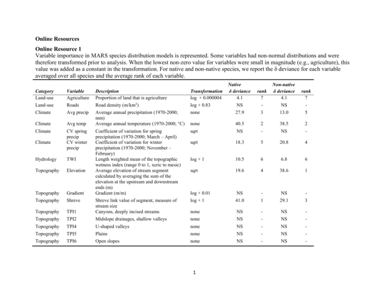
Variable importance in MARS species distribution models is represented. Some variables had non-normal distributions and were
therefore transformed prior to analysis. When the lowest non-zero value for variables were small in magnitude (e.g., agriculture), this
value was added as a constant in the transformation. For native and non-native species, we report the δ deviance for each variable
averaged over all species and the average rank of each variable.
Native
δ deviance
4.1
rank
7
Non-native
δ deviance
4.1
rank
7
Category
Land-use
Variable
Agriculture
Description
Proportion of land that is agriculture
Transformation
log + 0.000004
Land-use
Roads
Road density (m/km2)
log + 0.83
NS
-
NS
-
Climate
Avg precip
none
27.9
3
13.0
5
Climate
Avg temp
Average annual precipitation (1970-2000;
mm)
Average annual temperature (1970-2000; °C)
none
40.5
2
38.5
2
Climate
CV spring
precip
CV winter
precip
Coefficient of variation for spring
precipitation (1970-2000; March – April)
Coefficient of variation for winter
precipitation (1970-2000; November –
February)
Length weighted mean of the topographic
wetness index (range 0 to 1, xeric to mesic)
Average elevation of stream segment
calculated by averaging the sum of the
elevation at the upstream and downstream
ends (m)
Gradient (m/m)
sqrt
NS
-
NS
-
sqrt
18.3
5
20.8
4
log + 1
10.5
6
6.8
6
sqrt
19.6
4
38.6
1
log + 0.01
NS
-
NS
-
log + 1
41.0
1
29.1
3
none
NS
-
NS
-
Climate
Hydrology
TWI
Topography
Elevation
Topography
Gradient
Topography
Shreve
Topography
TPI1
Shreve link value of segment, measure of
stream size
Canyons, deeply incised streams
Topography
TPI2
Midslope drainages, shallow valleys
none
NS
-
NS
-
Topography
TPI4
U-shaped valleys
none
NS
-
NS
-
Topography
TPI5
Plains
none
NS
-
NS
-
Topography
TPI6
Open slopes
none
NS
-
NS
-
1
Online Resource 2
Spatial conservation prioritization approaches typically use species occurrence data to identify
high priority areas for management activity. The conservation prioritization program Zonation
(version 2.0 and 3.1) permits users to add complexity by incorporating positive or negative
interactions between species into the planning process. Here we describe how interactions
between native and non-native species were incorporated into our analysis to identify restoration
and preservation PAs for native fish conservation planning in the Gila River basin of the
Southwestern, USA.
For restoration PAs, a positive interaction was assigned for native species with nonnative species prioritizing areas of high overlap of the species distributions. For preservation
PAs, a negative interaction was assigned de-emphasizing areas of high overlap between the two
species types prioritizing areas with exclusively native species. Zonation determines the
interaction between species distributions by calculating the connectivity of species distribution
layers. We have outlined below the methodology utilized for applying species interactions into
our analysis (also see Moilanen and Kujala 2008).
The terms eij and fik represent the local occurrence of non-native species j and native
species k in grid cell i, respectively. Let βk be the parameter modeling the spatial scale of
potential stream travel distance for native species k. βk is the parameter of a negative exponential
function. We specify the interaction intensity of non-native species j at cell i by native species k
is Eij, which is the local non-native species occurrence multiplied by the connectivity of the cell
to the native species distribution, Sijk, using parameter βk to model the travel distance of the
native species (d in is distance between cells i and n). Thus locations with high Eij have the
occurrence of the non-native species well within the travel distance to the native species.
2
Essentially, Eq. (1) represents the positive association of the non-native species to the
distribution of the native species.
Restoration Priority Areas (Eq. 1)
S𝑖𝑗𝑘
∑𝑁
𝑛−1 exp(−𝛽𝑘 𝑑𝑖𝑛 ) 𝑓𝑛𝑘
𝐸𝑖𝑗𝑘 = e𝑖𝑗 min {1.0, max
} = e𝑖𝑗 min {1.0,
}
𝛾𝑗 max ∑𝑁
𝑛−1 exp(−𝛽𝑘 𝑑𝑖𝑛 ) 𝑓𝑛𝑘
𝛾𝑗
𝑆𝑖𝑗𝑘
𝑖
The interaction component between native and non-native species was then calculated for the
preservation PAs (Eq. 2) by specifying that the discounted value of feature j at cell i is Eij, which
is the local occurrence of the focal feature eij discounted by connectivity to the native species to
be avoided f, using parameter βk to model the distances to which the undesirable influence
spreads.
Preservation Priority Areas (Eq. 2)
S𝑖𝑗𝑘
∑𝑁
𝑛−1 exp(−𝛽𝑘 𝑑𝑖𝑛 ) 𝑓𝑛𝑘
𝐸𝑖𝑗𝑘 = e𝑖𝑗 min {1.0, max
} = e𝑖𝑗 min {1.0,
}
𝛾𝑗 max ∑𝑁
𝑛−1 exp(−𝛽𝑘 𝑑𝑖𝑛 ) 𝑓𝑛𝑘
𝛾𝑗
𝑆𝑖𝑗𝑘
𝑖
3
Online Resource 3
A map of the (a) Gila River basin within the American Southwest, USA, displaying the major
rivers, cities, dams, and basin boundaries (b) the top 10% of preservation and restoration PAs
overlaid with the species richness within each catchment (>1 species per catchment minimum to
capture community richness) from the original field records, and (c) a section of the mainstem
Verde River displaying species richness and the top PAs in the basin.
4