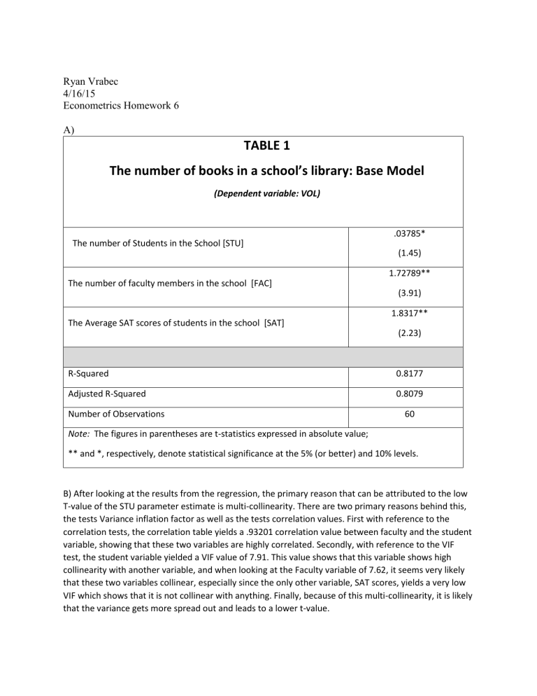
TABLE 1 The number of books in a school`s library: Base Model

Ryan Vrabec
4/16/15
Econometrics Homework 6
A)
TABLE 1
The number of books in a school’s library: Base Model
(Dependent variable: VOL)
The number of Students in the School [STU]
The number of faculty members in the school [FAC]
The Average SAT scores of students in the school [SAT]
.03785*
(1.45)
1.72789**
(3.91)
1.8317**
(2.23)
R-Squared
Adjusted R-Squared
0.8177
0.8079
Number of Observations
Note: The figures in parentheses are t-statistics expressed in absolute value;
60
** and *, respectively, denote statistical significance at the 5% (or better) and 10% levels.
B) After looking at the results from the regression, the primary reason that can be attributed to the low
T-value of the STU parameter estimate is multi-collinearity. There are two primary reasons behind this, the tests Variance inflation factor as well as the tests correlation values. First with reference to the correlation tests, the correlation table yields a .93201 correlation value between faculty and the student variable, showing that these two variables are highly correlated. Secondly, with reference to the VIF test, the student variable yielded a VIF value of 7.91. This value shows that this variable shows high collinearity with another variable, and when looking at the Faculty variable of 7.62, it seems very likely that these two variables collinear, especially since the only other variable, SAT scores, yields a very low
VIF which shows that it is not collinear with anything. Finally, because of this multi-collinearity, it is likely that the variance gets more spread out and leads to a lower t-value.
TABLE 2
The number of books in a school’s library: With Linear Student to teacher variable
(Dependent variable: VOL)
Linear Combination of Students and Faculty (TOT)
The Average SAT scores of students in the school [SAT]
.08735**
(12.87)
.83656**
(2.02)
R-Squared
Adjusted R-Squared
Number of Observations
0.8052
0.7984
60
Note: The figures in parentheses are t-statistics expressed in absolute value;
** and *, respectively, denote statistical significance at the 5% (or better) and 10% levels.
Part (E) Post Hetero-skedasticity tests;
Linear Combination of Students and Faculty (TOT)
The Average SAT Scores of Students in the School (SAT)
.08735**
(4.92)
1.69003**
(2.44)
Note: The figures in parentheses are t-statistics expressed in absolute value;
** and *, respectively, denote statistical significance at the 5% (or better) and 10% levels.
C) After creating a linear combination of students to faculty and combining that with SAT scores, this new model is much better. There are a couple reasons that this model is better, the first and foremost being that (assuming the above test had collinear variables) the new model accounted for the multi
collinearity within the data set. By combining the faculty and student variables, the new model generates two variables with statistically significant t-values, of which the TOT variable is extremely high with a value of 12.87. Secondly, when looking at the R-squared values, while the second model does yield a value that is slightly lower than the first model, it is also using one less variable and only losing around one percent of the models explanatory power, which means that overall the model is stronger.
D)
After plotting the residuals and looking at the differences in t-values after running the White test with the regression, it is possible to say that both of the variables are heteroskedastic. The reason being that with reference to the residual plot, you can see that as the X-value continues to grow, the variance with the plots is not by any means constant in either of the variables. In addition, when looking at the regression results with the white test, there are some noticable differences in t-values, most especially with the TOT variable in which the t-value falls from nearly 12.87 to 4.92. This much of a change after running a test that accounts for heteroskedasticity shows that there were some heteroskedastic qualities to the data.
E) After re-running the model and correcting for hetero-skedasticity, there is a notable difference in the t-values of the (TOT) variable, as it dropped from 12.87 to 4.92. In addition there was a slight change in the value of the (SAT) value in which it rose from 2.02 to 2.44 after being corrected for heteroskedasticity. Overall after the hetero-skedastic corrections both values have different t-values, but nonetheless are both still statiscally signifigant.
Question 5 (pg 269)
Answer) A
The reason I believe the answer is (A) is because they are two variables that would closely allign witheachother and would likely be affected in the same way by many market shortcomings. In addition the other options don’t seem like they would hold constant with eachother. In option (B) The price of refridgerators and the price of washing machine could vary from eachother depending on several factors. In option (C) the amount of a crop harvest can vary to largely from the amount of seed used due to labor values, weather conditions or things such as price of fertilizer. Finally option (D) doesn’t seem to make sense because interest rates and money supply are only dependent on eachother in the short run not the long run.
Question 11 (pg 272)
A)
M= positive (M>0) The reason that this variable would be assumed to be positive is that with a higher admission test score, it shows that the student is more qualified to be at that school and is prepared to work hard and achieve at the business school.
B= positive (B>0) The reason that this variable would be assumed to be positive is that years of experience in the field would yield some positive effects on the students scores, because they would understand some of the real world application of the work they are doing, and also be more likely to understand how important a graduate degree is as far as an attribute that allows you to advance further in their career.
A= negative (A<0) The reason that this variable would be assumed to be negative, is that with an older age value, intuition would show that those students had spent more time out of school since they completed their undergraduate degree meaning that they would be likely to forget some of the imformation that would be found more vaulable in academia than in real world application.
S= positive (S>0) The reason that this variable would be assumed to be positive is that an undergraduate education in Economics would definitly help a student in understnading business structure, both at the micro and macro level. This in turn would help with the students studies and could lead to a higher GPA.
B)
A problem with this regression is that the age variable and experience variable counter eachother and could be multi-collinear. The reason being that in order to gain work experience the student would have had to spend time outside of school, whereas those with no work experience may be younger upon entrance to the business school but are missing out on the work experience that could benefit them. In addition, with regard to the S value, there could also be other under graduate degrees included such as finance, marketing or business that could also benefit a student going into the graduate school of business. By including these, the results would likely change the overall GPA value.
C)
My reaction to the idea of a suggestion to making the A variable into a polynomial functional form would be agreeable. By allowing the Age variable to be changed into a polynomial form, the regression could better estimate the effect of age without simply basing it down to a year by year basis.
Yes, there would likely be a statistical difference between a 22 year old and a 32 year old, but the overall difference between a 32 year old and a 34 year old in terms of experience and overall ability is probably negligible. By allowing for variable A to be turned into polynomial form, the regression results will be more accurate.
D)
In addition to making the age variable polynomial and expanding the S varibale to include other undergraduate degrees, one way to improve the model would be to include variables such as undergraduate GPA, or what the students GPA was in business realted classes. In addition to those,
another variable that could be added is whether or not the student had an undergraduate internship, this would likely give him or her experience in the field, but usually only a semester or two, not enough to be measured in year terms of the experience variable above.
Code; data one; set WORK.Homework6;
TOT= FAC* 10 +STU; proc reg ; title 'basic model' ; model VOL = STU FAC SAT; run ; proc reg ; title 'linear students and faculty' ; model VOL= TOT SAT; run ; proc reg ; title 'basic model with white test+vif' ; model VOL = STU FAC SAT/ white vif ; run ; proc reg ; title ' runnning student linear model with white test' ; model VOL= TOT SAT/ white ; run ; proc corr ; run ;


