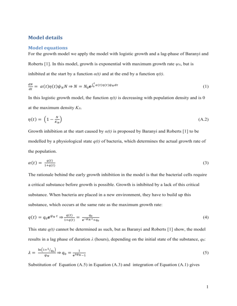
Model details
Model equations
For the growth model we apply the model with logistic growth and a lag-phase of Baranyi and
Roberts [1]. In this model, growth is exponential with maximum growth rate ψN, but is
inhibited at the start by a function α(t) and at the end by a function η(t).
𝑑𝑁
𝑑𝑡
𝑡
= 𝛼(𝑡)𝜂(𝑡)𝜓𝑁 𝑁 ⇒ 𝑁 = 𝑁0 𝐞∫0 𝛼(𝜏)𝜂(𝜏)𝜓𝑁 𝑑𝜏
(1)
In this logistic growth model, the function η(t) is decreasing with population density and is 0
at the maximum density KN.
𝑁
𝜂(𝑡) = (1 − 𝐾 )
(A.2)
𝑁
Growth inhibition at the start caused by α(t) is proposed by Baranyi and Roberts [1] to be
modelled by a physiological state q(t) of bacteria, which determines the actual growth rate of
the population.
𝛼(𝑡) =
𝑞(𝑡)
(3)
1+𝑞(𝑡)
The rationale behind the early growth inhibition in the model is that the bacterial cells require
a critical substance before growth is possible. Growth is inhibited by a lack of this critical
substance. When bacteria are placed in a new environment, they have to build up this
substance, which occurs at the same rate as the maximum growth rate:
𝑞(𝑡)
𝑞(𝑡) = 𝑞0 𝐞𝜓𝑁 𝑡 ⇒ 1+𝑞(𝑡) =
𝑞0
𝐞−𝜓𝑁 𝑡 +𝑞0
(4)
This state q(t) cannot be determined as such, but as Baranyi and Roberts [1] show, the model
results in a lag phase of duration λ (hours), depending on the initial state of the substance, q0:
𝜆=
ln(1+1⁄𝑞0 )
𝜓𝑁
1
⇒ 𝑞0 = 𝐞𝜆𝜓𝑁 −1
(5)
Substitution of Equation (A.5) in Equation (A.3) and integration of Equation (A.1) gives
1
𝑑𝑁
𝑑𝑡
=
𝐞𝜓𝑁 𝑡
𝐞𝜓𝑁 𝜆 +𝐞𝜓𝑁 𝑡 −1
𝜓𝑁 𝑁 (1 −
𝑁
𝐾𝑁
)⇒𝑁 =
𝐾𝑁 𝑁0 (𝐞𝜓𝑁 𝜆 +𝐞𝜓𝑁 𝑡 −1)
𝐾𝑁 𝐞𝜓𝑁 𝜆 +𝑁0 (𝐞𝜓𝑁 𝑡 −1)
(6)
This growth model is now used for more than one bacterial population (Donor D, Recipient R
and Transconjugant T) by adding conjugation terms γ and plasmid loss terms ξ in the
differential equations:
𝑑𝑅
𝑑𝑡
𝑑𝑇
𝑑𝑡
𝑑𝐷
𝑑𝑡
𝐞𝜓𝑅 𝑡
𝑅
= 𝐞𝜓𝑅𝜆+𝐞𝜓𝑅𝑡−1 𝜓𝑅 𝑅 (1 − 𝐾 ) − 𝛾𝑅(𝑇 + 𝐷) + 𝜉𝑇
𝑅
𝐞𝜓𝑇 𝑡
𝑇
= 𝐞𝜓𝑇𝜆 +𝐞𝜓𝑇𝑡−1 𝜓𝑇 𝑇 (1 − 𝐾 ) + 𝛾𝑅(𝑇 + 𝐷) − 𝜉𝑇
𝑇
𝐞𝜓𝐷 𝑡
𝐷
= 𝐞𝜓𝐷𝜆 +𝐞𝜓𝐷𝑡 −1 𝜓𝐷 𝐷 (1 − 𝐾 )
𝑁 =𝑅+𝑇+𝐷
𝐷
(7)
(8)
(9)
(10)
2
Table 1 Overview of model symbols
Symbol
Unit
Description
R
cfu/ml
Recipient concentration
D
cfu/ml
Donor concentration
T
cfu/ml
Transconjugant concentration
N
cfu/ml
Total bacterial concentration
ψ
h-1
Intrinsic growth rate
K
cfu/ml
Maximum density
λ
h
Lag phase
N0, R0,T0, D0
cfu/ml
Initial concentration
γD, γT
bacterium-1 h-1
Conjugation rates
ξ
bacterium-1 h-1
Plasmid loss rate
σ
-
Plasmid loss constant in continuous
segregation model (CS model)
ρ
bacterium-1 h-1
Plasmid loss constant in densitydependent segregation model (DS model)
3
Derivation of the equations for estimation of plasmid loss parameters
The fraction of bacteria carrying the plasmid p is given by
𝑝 = 𝑇⁄𝑁
𝑑𝑝
𝑑𝑡
𝑑𝑝
𝑑𝑡
=
𝑑(𝑇 ⁄𝑁 )
𝑑𝑡
(B.1)
=
𝑇′
𝑁
−
𝑇𝑁′
(B.2)
𝑁2
= 𝛾 𝑁𝑝 (1 − 𝑝) − 𝜉𝑝
(B.3)
The initial fraction p0 in the experiment from which plasmid loss was estimated, is 1, because
we started with an initial population of T only. Assuming that the fraction of bacteria without
plasmids remains very low, we can ignore conjugation and Equation (B.3) becomes
𝑑𝑝
𝑑𝑡
= −𝜉𝑝
(B.4)
For the CS model with constant plasmid loss at rate σ, the fraction of the population p will
decrease at a constant rate and starts with only plasmid carrying bacteria, p0 =1
𝑝(𝑡) = 𝐞−𝜎𝑡 .
(B.5)
This σ can be estimated by
1
𝜎 = − 𝑡 𝑙𝑛(𝑝(𝑡)).
(B.6)
For the DS model with density-dependent plasmid loss, we assume that the loss of plasmids is
related to the growth rate of the population. The rationale is that plasmid loss occurs during
cell division in which one of the daughter cells does not receive the plasmid. The equation for
the change in the fraction of the population p of bacteria carrying plasmids for the DS model
is given by
𝑑𝑝
𝑑𝑡
= 𝜎𝛼(𝑡)𝜂(𝑡)𝜓𝑝
(B.7)
The fraction p will decrease with the growth of the population
𝑡
𝑝(𝑡) = 𝑝0 𝐞−𝜎 ∫0 𝜓 𝛼(𝜏)𝜂(𝜏)𝑑𝑡
(B.8)
Because p0 = 1 and from Equation A.6 we know that the total bacterial population can be
𝑡
described by 𝑁(𝑡) = 𝑁0 𝐞∫0 𝛼(𝜏)𝜂(𝜏)𝜓𝑁 𝑑𝜏 , Equation (B.8) can be written as
4
𝑝(𝑡) = 𝑁(𝑡)⁄𝑁0 𝐞−𝜎
(B.9)
The parameter σ can then be estimated as
𝜎 = ln 𝑁(𝑡)⁄𝑁0 − ln 𝑝 (𝑡)
(B.10)
Model fitting algorithm
The model was fitted by the NonlinearModelFit method of Mathematica (version 8.0.1.0,
Wolfram Research Inc.). This is based on the least squares method and minimization of the
sum of squares was done with the Levenberg-Marquardt algorithm. The NonlinearModelFit
method provided the confidence intervals and AICc values form which we calculated the
adjusted Akaikes Information Criterium (AICc):
𝐴𝐼𝐶𝑐 = 𝐴𝐼𝐶 +
2 𝑘 (𝑘+1)
𝑛−𝑘−1
(C.1)
in which k is the number of parameters and n is the number of samples.
References
1.
Baranyi J, Roberts TA: A Dynamic Approach to Predicting Bacterial-Growth in
Food. Int J Food Microbiol 1994, 23(3-4):277-294.
5