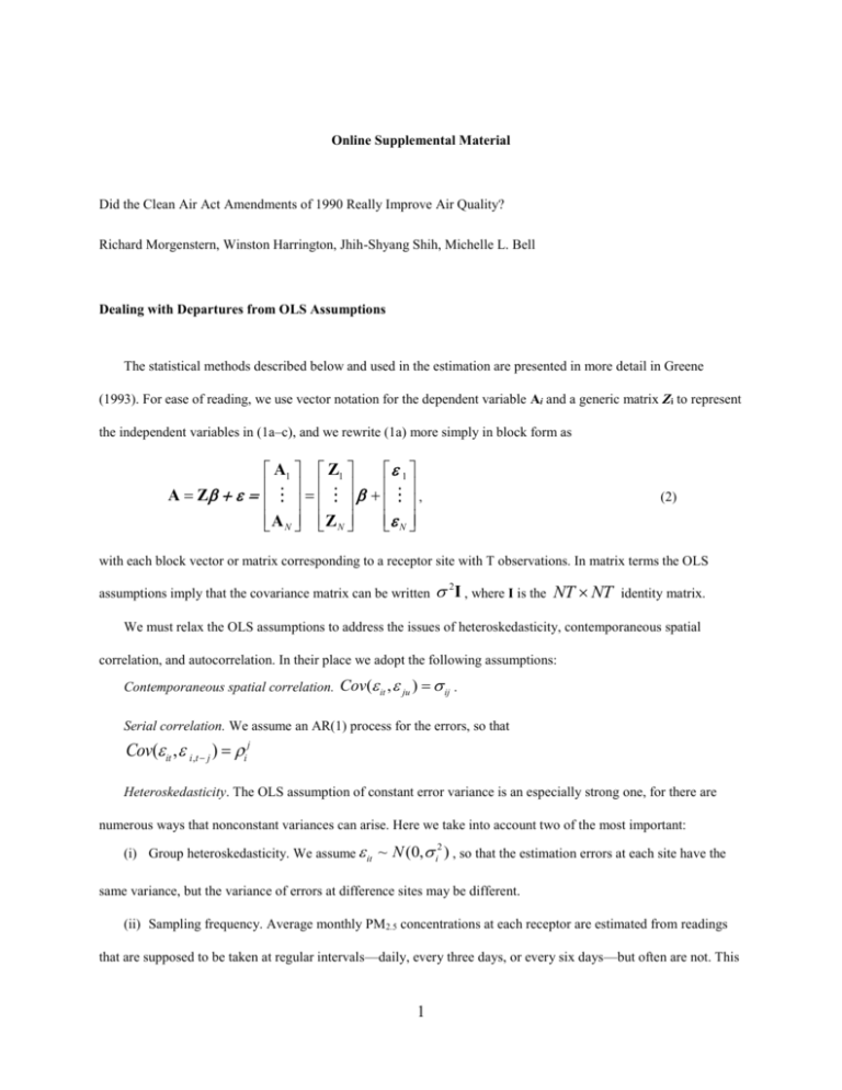
Online Supplemental Material
Did the Clean Air Act Amendments of 1990 Really Improve Air Quality?
Richard Morgenstern, Winston Harrington, Jhih-Shyang Shih, Michelle L. Bell
Dealing with Departures from OLS Assumptions
The statistical methods described below and used in the estimation are presented in more detail in Greene
(1993). For ease of reading, we use vector notation for the dependent variable Ai and a generic matrix Zi to represent
the independent variables in (1a–c), and we rewrite (1a) more simply in block form as
 A1   Z1 
 1 




A  Z             ,
 A N   Z N 
 N 
(2)
with each block vector or matrix corresponding to a receptor site with T observations. In matrix terms the OLS
assumptions imply that the covariance matrix can be written
 2I , where I is the NT  NT
identity matrix.
We must relax the OLS assumptions to address the issues of heteroskedasticity, contemporaneous spatial
correlation, and autocorrelation. In their place we adopt the following assumptions:
Contemporaneous spatial correlation. Cov( it ,  ju )   ij .
Serial correlation. We assume an AR(1) process for the errors, so that
Cov( it ,  i ,t  j )  i j
Heteroskedasticity. The OLS assumption of constant error variance is an especially strong one, for there are
numerous ways that nonconstant variances can arise. Here we take into account two of the most important:
(i) Group heteroskedasticity. We assume  it ~ N (0,  i ) , so that the estimation errors at each site have the
2
same variance, but the variance of errors at difference sites may be different.
(ii) Sampling frequency. Average monthly PM2.5 concentrations at each receptor are estimated from readings
that are supposed to be taken at regular intervals—daily, every three days, or every six days—but often are not. This
1
means that the number of daily readings in a month can vary from 1 to 31, and for that reason the precision of
monthly estimates will differ greatly for different months even at the same site.
We deal with sampling frequency first, and then everything else in a single step.
Sampling frequency. As discussed above, in Section 2, most of the receptors in the sampling network had
periods when very few daily measurements were being made. To obtain a balanced panel, we were forced to use
such receptors; if we had not, we would have had very few receptors with which to do the analysis. Rather than
discard a receptor, it was better to discount the importance of the months that had only a few daily observations.
The correction is based on the well-known formula for the variance of a sample mean. If
Aiym   diymj Niym
in (1a–c) is the mean of N iym daily observations, which we assume to be independent and
identically distributed, then var( Aiym )  var(dij ) / N iym is the sampling variance of the Aiym . We can correct for
the nonconstant sampling variance by weighting the observations by either the monthly variance directly or the
number of observations for the month. It turns out that weighting by the number of monthly observations is far
superior because it guarantees that months at individual monitors with few observations get small weights. Using the
monthly variance gives too much weight to months with very few observations that happen to be very close in
magnitude.
Therefore, in the first step of the estimating procedure we transform (2) to
N .* A  N .* Z  N .*  ,
where
(2a)
N is a column vector containing the square root of the number of daily observations in each monthly
estimate, and .* the operation of pairwise multiplication.
Correcting for contemporaneous spatial correlation, serial correlation, and group heteroskedasticity. If Z
represents the complete matrix of independent variables in (1a) and
then the errors
ˆ
the vector of coefficients estimated by OLS,
eit  Ait  Zˆ it for t=1,…,T. The error structure of (2) is now
 11
V  
N 1
1N 

,
NN 
where
2
(3)
1
 j  2j


1
j
 ij  i2

ij 
i 1
1  i  j  i

  T 1
 i
i
 Tj 1 

 Tj  2 



1 
(4)
OLS cannot be used to estimate the models (1a–1c) with the error structure in (3) and (4). Instead, we use
feasible generalized least squares (FGLS) and maximum likelihood (ML) (Greene 1993). These methods are
asymptotically equivalent but can give very different results in small samples. With our relatively large data set, we
find the results are quite similar for the two estimation methods.
The generalized least squares estimator for the model is
   ZT V 1Z  ZT V 1A .
1
To estimate (5) we need estimates for the parameters in each
ij in (4). The basic strategy is to estimate
(1a) using OLS and use the OLS residuals to estimate the site-level error variances
coefficients
(5)
 i2 and the autocorrelation
i . Denoting the OLS residuals by eit , our estimates of these parameters are
sii  si2 
1
 eit ei (t 1)
eit2 and ri 

(T  1) si2 ,
T t
(6)
respectively.
Contemporaneous Spatial Correlation
Unfortunately, we cannot use a similar method to obtain estimates of the covariance terms in (4) because
too many covariances are required. Although we can compute the sample covariance for any two sites by
sij   eit e jt / T , the matrix sij
would not be of full rank. With 193 receptors and 84 months of data, we would
have 18,528 covariance terms to estimate and only 16,212 observations. We use the fact that the observed
correlations are strongly related to distance to estimate a simple model of covariance. That is, we specify that the
error covariance between sites i and j depends on the error variances at each site and an exponential function of the
distance D (i, j ) between them, and we estimate this covariance
 ij by
sij  si s j exp   2 D  i, j   .
3
(7)
Then we estimate the decay coefficient  by finding the best least squares fit to the site-level empirical
correlations. The expressions in (6) and (7) give us everything we need to produce a FGLS estimator of the  . The
same expressions also provide the starting values for estimates of the σs and the s in the maximum likelihood
estimation (MLE).
4
Using Estimated Coefficients to Generate Counterfactuals
To generate a set of n random draws from a common normal distribution N (  , ) , we draw a set of n
2
standard normal variables ui , where ui ~N(0,1), and the desired set of random draws is xi     ui . For a
multivariate normal random variable coefficient vector
The parameter vector


has the distribution N

as in (5) above, the procedure is analogous.
  ,Var    , where Var (  ) is the covariance matrix of
. Because Var(  ) is positive definite, it can be written as CCT , where C is a matrix whose columns are the
characteristic vectors of Var(  ) and  is a matrix that has the (all positive) characteristic roots along the diagonal
and zeros elsewhere. Now if we draw a standard normal vector u
dimensionality as

, then the vector x 


uT  (u1, u2, ,..., uk ) , with the same

  C  u has the required distribution N  ,Var   
5
