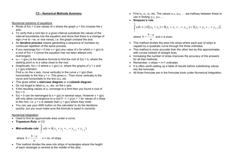
 Find x0, x1, x2, etc. The values x1/2, x3/2, … are halfway between these to
use in finding y1/2, y3/2, …
 Simpson’s rule:
C3 – Numerical Methods Summary
Numerical solutions of equations
 Roots of f(x) = 0 are values of x where the graph y = f(x) crosses the x
axis.
 To verify that a root lies in a given interval substitute the values of the
interval boundaries into the equation and show that there is a change of
sign (+ve to –ve, or vice versa), i.e. the graph crossed the axis.
 An iterative process means generating a sequence of numbers by
continued repetition of the same process.
 If you rearrange f(x) = 0 into x = g(x) any value of x for which x = g(x) is
a root of f(x) = 0 (since the equation has not been altered only
rearranged).
 xn+1 = g(xn) is the iterative formula to find the root of f(x) = 0, where the
starting point x0 is a value close to the root.
 Graphically: f(x) = 0 where x = g(x) i.e. where the graphs of y = x and
y = g(x) intersect.
Find x0 on the x axis, move vertically to the curve y = g(x) then
horizontally to the line y = x. This gives x1. Then move vertically to the
curve and horizontally to the line (x2), etc.
 This gives either a staircase diagram or a cobweb diagram.
 Do not forget to label x0, x1, etc. on the x axis.
 If the resulting values of xn converge to a limit then you found a root of
f(x) = 0.
 f(x) = 0 can be rearranged to x = g(x) in several ways. However x = g(x)
will only allow convergence to a root if –1 < g’(x) < 1 for values of x close
to the root. I.e. y = x is steeper than y = g(x) where they meet.
 You can use your ANS button on the calculator to do the iterations
quickly, but you must make sure the formula is typed in correctly.
Numerical integration
 Used to find an approximate area under a curve.
 Trapezium Rule: in C2
b
 Mid-ordinate rule:
 ydx  h( y
1
2
 y 3  ...  yn 3  yn 1 )
2
2
2
a
where h 
ba
n
n = no. of strips
 This method divides the area into strips of rectangles where the height
of each rectangle is centred at the middle of the strip.
b
 ydx  h( y
1
3
0
 yn )  4( y1  y3  ...  yn1 )  2( y2  y4  ...  yn2 ),
a
where h 
ba
and n is even.
n
 This method divides the area into strips where each pair of strips is
capped by a quadratic curve through the three ordinates.
 This method is more accurate than the other two as this approximates
with curves instead of straight lines.
 Increasing the number of strips improves the accuracy of the answers
for all tree methods.
 Remember: n strips = n+1 ordinates
 It is often worth setting up a table of results before substituting values
into the formulae.
 All three formulae are in the formulae book under Numerical Integration.