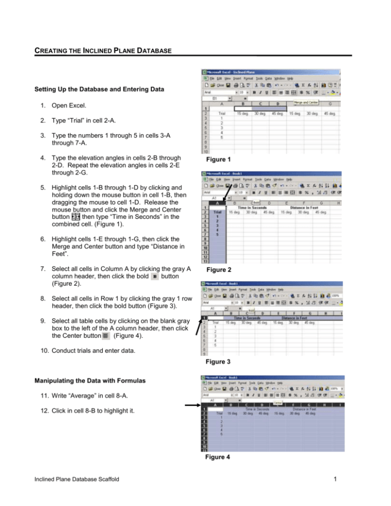
CREATING THE INCLINED PLANE DATABASE
Setting Up the Database and Entering Data
1. Open Excel.
2. Type “Trial” in cell 2-A.
3. Type the numbers 1 through 5 in cells 3-A
through 7-A.
4. Type the elevation angles in cells 2-B through
2-D. Repeat the elevation angles in cells 2-E
through 2-G.
Figure 1
5. Highlight cells 1-B through 1-D by clicking and
holding down the mouse button in cell 1-B, then
dragging the mouse to cell 1-D. Release the
mouse button and click the Merge and Center
button
then type “Time in Seconds” in the
combined cell. (Figure 1).
6. Highlight cells 1-E through 1-G, then click the
Merge and Center button and type “Distance in
Feet”.
7. Select all cells in Column A by clicking the gray A
column header, then click the bold
button
(Figure 2).
Figure 2
8. Select all cells in Row 1 by clicking the gray 1 row
header, then click the bold button (Figure 3).
9. Select all table cells by clicking on the blank gray
box to the left of the A column header, then click
the Center button
(Figure 4).
10. Conduct trials and enter data.
Figure 3
Manipulating the Data with Formulas
11. Write “Average” in cell 8-A.
12. Click in cell 8-B to highlight it.
Figure 4
Inclined Plane Database Scaffold
1
13. Click the = sign (Figure 5).
14. Select “Average” from the drop down menu
(Figure 6). Note that Excel enters the data
cells 3-B through 7-B in the formula line
automatically. You can use this feature to
double check that Excel is performing the
correct calculation on the correct cells. Click
OK.
15. Add averages for the remaining data columns
by highlighting cell 8-B and selecting Copy from
the Edit drop down menu, then click on 8-C
and select Paste. To do this more easily, you
can also use the shortcut keys: use Ctrl C for
copy and Ctrl V for paste. Add averages for
cells 8-D through 8-G.
Figure 5
16. Write “Speed (ft/sec)” in cell 9-A. Adjust the
width of the cell so that the entire label is visible
by either double clicking the right-hand column
divider or left-clicking the mouse on the column
divider then dragging the column boundary to
the desired position and releasing the mouse
button.
Figure 6
17. Click in cell 9-B to highlight it.
18. Click on the = sign, then click on cell 8-E; note
that Excel enters the cell location in the formula
line automatically. Write the symbol for divide
“/”, then click on cell 8-B. Note that Excel
writes the formula both in the formula line and
in cell 9-B (Figure 7). You can use this feature
to double check that Excel is performing the
correct calculation on the correct cells. Click
OK.
19. Add formulas in cells 9-C and 9-D to find the
average speeds at the other ramp angles by
repeating the formula building steps described
in 17 and 18 using the appropriate cells.
Figure 7
20. Truncate the formula results to two decimal
places by first clicking in cell 9-B to highlight it.
Then go to Cells on the Format drop down
menu. On the number tab, select Number.
Select 2 decimal places (Figure 8) and click
OK.
21. Repeat for cells 9-C and 9-D.
Figure 8
Inclined Plane Database Scaffold
2
Graphing the Data
22. Click on the Chart Wizard
button.
23. Create a Scatter Plot by selecting “XY
(Scatter)” as the chart type, then selecting
“Scatter” as the Chart sub-type and clicking
Next (Figure 9).
24. Select the data range to be graphed by clicking
cell 3-B, holding the mouse button and
dragging to cell 7-G, then releasing the mouse
button (Figure 10). Do NOT click Next. As
selected, the data will not produce the graph
most useful for analyzing the results. Doing so
requires specifying more exactly how to create
the graph, as described in steps 25 through 28.
Figure 9
25. Select the Series tab. Clear the data by
clicking the Remove button until all the series
are removed (Figure 11).
26. Click the Add button. Add the data for 15
degrees by clicking in the Name field and
typing “15 Degrees”. Press the Tab key to
move to the next field. Choose the X axis data
by clicking cell 3-B, holding the mouse button
and dragging to cell 7-B. Press the Tab key
and choose the Y axis data by clicking cell 3-E,
holding the mouse button and dragging to cell
7-E (Figure 12).
Figure 10
27. Add the data for 30 degrees by repeating step
26 using the cells 3-C to 7-C for the X axis data
and cells 3-F to 7-F for the Y axis data.
28. Add the data for 45 degrees by repeating step
26 using cells 3-D to 7-D for the X axis data
and cells 3-G to 7-G for the Y axis data. Click
the Next button.
Figure 11
Figure 12
Inclined Plane Database Scaffold
3
29. Type the title “Distance - Time Results” in the
Chart Title box. Press the Tab key to move to
the next field. Type “Time in Seconds” for the
X axis value. Press the Tab key and type
“Distance in Feet” for the Y axis value, then
click Next (Figure 13).
30. Select “As object in Sheet 1” and click Finish.
(Figure 14).
Figure 13
31. Move the graph under the data (Figure 15).
Note that the data points on the graph are all
bunched together making them hard to read.
Make them easier to read by changing the
scales as described in step 32.
32. Change the Y axis scale by double clicking the
numbers on the Y axis (Figure 15). On the
scale tab, double click in the minimum field and
enter 8. Double click in the maximum field and
enter 18. Click OK (Figure 16).
Figure 14
33. Change the X axis scale by double clicking the
numbers on the X axis. On the scale tab,
double click in the minimum field and enter 4.
Double click in the maximum field and enter 8.
Click OK.
Exporting the Results
34. Open Word by going to the Start button in the
lower left corner of the screen, selecting
Programs, then Word.
35. Write your name, then cut and paste the chart
you’ve created into the document.
36. Write the question the experiment was
designed to answer, your initial hypothesis,
then describe the results of the experiment as
reflected by the average speed results and the
Distance - Time chart. Finally, write how you
explain the results and your ideas for
additional experiments.
Figure 15
37. Format your final document, then print it.
Figure 16
Inclined Plane Database Scaffold
4