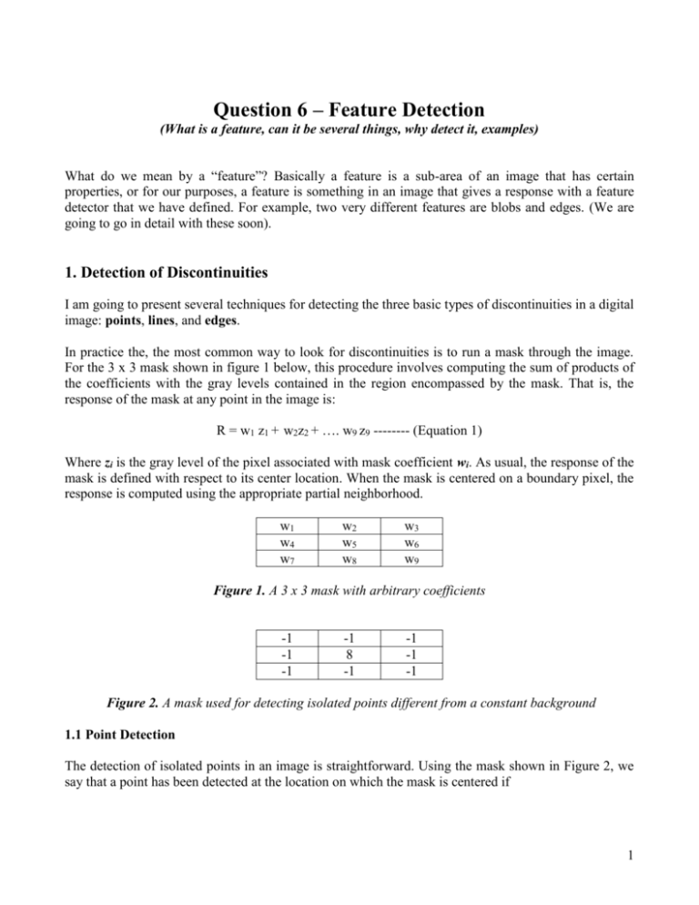
Question 6 – Feature Detection
(What is a feature, can it be several things, why detect it, examples)
What do we mean by a “feature”? Basically a feature is a sub-area of an image that has certain
properties, or for our purposes, a feature is something in an image that gives a response with a feature
detector that we have defined. For example, two very different features are blobs and edges. (We are
going to go in detail with these soon).
1. Detection of Discontinuities
I am going to present several techniques for detecting the three basic types of discontinuities in a digital
image: points, lines, and edges.
In practice the, the most common way to look for discontinuities is to run a mask through the image.
For the 3 x 3 mask shown in figure 1 below, this procedure involves computing the sum of products of
the coefficients with the gray levels contained in the region encompassed by the mask. That is, the
response of the mask at any point in the image is:
R = w1 z1 + w2z2 + …. w9 z9 -------- (Equation 1)
Where zi is the gray level of the pixel associated with mask coefficient wi. As usual, the response of the
mask is defined with respect to its center location. When the mask is centered on a boundary pixel, the
response is computed using the appropriate partial neighborhood.
w1
w4
w7
w2
w5
w8
w3
w6
w9
Figure 1. A 3 x 3 mask with arbitrary coefficients
-1
-1
-1
-1
8
-1
-1
-1
-1
Figure 2. A mask used for detecting isolated points different from a constant background
1.1 Point Detection
The detection of isolated points in an image is straightforward. Using the mask shown in Figure 2, we
say that a point has been detected at the location on which the mask is centered if
1
R  T -------------------- (Equation 2)
Where T is a nonnegative threshold, and R is given by equation 1. Basically, all that this formulation
does is measure the weighted differences between the center point and its neighbors. The idea is that
the gray level of an isolated point will be quite different from the gray level of its neighbors.
1.2 Line Detection
The next level of complexity involves the detection of lines in an image. Consider the masks shown in
Figure 3.
2
-1
-1
2
-1
-1
2
-1
-1
-1
2
-1
2
-1
2
-1
-1
-1
-1
-1
2
2
2
-1
-1
-1
2
-1
2
-1
-1
-1
2
-1
(a)
(b)
(c)
-1
-1
(d)
Figure 3. Line masks (a) Horizontal (b) +45o (c) Vertical (d) -45o
If the first mask were moved around an image, it World respond more strongly to lines (one pixel
thick) oriented horizontally. With constant background, the maximum response would result when the
line passed through the middle row of the mask. This is easily verified by sketching a simple array of
1’s with a line of a different gray level (say 5s) running horizontally through the array.
1.3 Edge Detection
Edge detection is by far the most common approach for detecting meaningful discontinuities in gray
level.
An edge is the boundary between two regions with relatively distinct ray-level properties.
Basically the idea underlying most edge-detection techniques is the computation of a local derivative
operator. Figure 4 illustrates this concept. Figure 4(a) shows an image of a light stripe on a dark
background, the gray-level profile along a horizontal scan line of the image, and the first and second
derivatives of the profile.
2
(a)
(b)
Figure 4. Edge detection by derivative operators; (a) light stripe on a dark background; (b) dark stripe
on a light background.
Note from the profile that an edge (transition from dark to light) is modeled as a smooth, rather than an
abrupt, change of gray level. This model reflects the fact that edges in digital images are generally
slightly blurred as a result of sampling.
Figure 4(a) shows that the first derivative of the gray level profile is positive at the leading edge of a
transition, negative at the trailing edge, and as expected, zero in areas of constant gray level. The
second derivative is positive for that part of the transition associated with the dark side of the edge,
negative for the part of the transition associated with the light side of the edge, and zero in areas of
constant gray level. Hence the magnitude of the first derivative can be used to detect the presence of an
edge in an image, and the sign of the second derivative can be used to determine whether an image
pixel lies on the dark or light side of an edge.
3
The first derivative at any point in an image is obtained by using the magnitude of the gradient at that
point. The second derivative is similarly obtained by using the Laplacian.
Gradient Operators  The gradient of an image f(x, y) at location (x, y) is the vector
 f 
 G   x 
 f   x     --------------------- (Equation 3)
 G y   f 
 y 
It is well known from vector analysis that the gradient vector points in the direction of maximum rate
of change of f at (x, y). In edge detection an important quantity is the magnitude of this vector,
generally referred to simply as the gradient and denoted f , where:
f = mag(  f) = [Gx2 + Gy2]1/2 ----------------------- (Equation 4)
Common practice is to approximate the gradient with absolute values:
f  G x  G y ----------------------------- (Equation 5)
The direction of the gradient vector also is an important quantity. Let α(x, y) represent the direction
angle of the vector  f at (x, y). Then from vector analysis:
 Gy
α(x, y)  tan 1 
 Gx

 ------------------- (Equation 6)

where the angle is measured with respect to the x-axis.
4
Example  Figure 5(a) [Figure 7.6(a)] shows an original image, and Figure 5(b) shows the result of
computing G x with the mask shown in Figure 6(a) [Figure 7.5(b)]. The x-axis are defined in the
vertical direction thus the strongest response produced by G x is expected to be on edges perpendicular
to the x-axis. This result is obvious in Figure 5(b), which shows strong responses along horizontal
edges, such as the river bank. Note also the relative lack of response along vertical edges. The reverse
situation occurs upon computation of G y , as Figure 5(c) shows. Combining these two results via
Equation 5 yielded the gradient image shown in Figure 5(d).
Figure 5. (a) Original image; (b) result of applying the mask in figure 6(a) to obtain Gx; (c) Result of
using the mask in Figure 6 (b) to obtain Gy; (d) Complete gradient image
5
-1
0
1
-2
0
2
-1
0
1
0
0
0
1
2
1
(a)
-1
-2
-1
(b)
Figure 6. Mask used to compute Gx at center point of the 3 x 3 region; (b) mask used to compute Gy at
that point
Laplacian  The Laplacian of a 2-D function f(x, y) is a second-order derivative as
2 f 
2 f 2 f
------------------------ (Equation 7)

x 2 y 2
The basic requirement in defining the digital Laplacian is that the coefficient associated with the centre
pixel be positive and the coefficients associated with the outer pixels be negative (high-pass filter
mask).
Laplacian is seldom used in practice for edge detection for several reasons. As a second order
derivative, the Laplacian typically is unacceptably sensitive to noise. Moreover, the Laplacian produces
double edges (figure 4) and is unable to detect edge direction. For these reasons, the Laplacian usually
plays the secondary role of detector for establishing whether a pixel is on the dark or light side of an
edge.
(Can also mention zero-crossing property of Laplacian which is used to find the location of edges)
2. Edge Linking and Boundary Detection
So far the techniques we have discussed detect intensity discontinuities. Ideally, these techniques
should yield pixels lying only on the boundary between regions. In practice, this set of pixels seldom
characterizes a boundary completely because of noise, breaks in the boundary from nonuniform
illumination, and other effects that introduce spurious intensity discontinuities. Thus edge detection
algorithms typically are followed by linking and other boundary detection procedures designed to
assemble edge pixels into meaningful boundaries. Several techniques are suited to this purpose.
2.1 Local Processing
One of the simplest approaches for linking edge points is to analyze the characteristics of pixels in a
small neighborhood (say, 3 x 3 or 5 x 5) about every point (x, y) in an image that has undergone edgedetection. All points that are similar are linked, forming a boundary of pixels that share some common
properties.
6
The two principle properties used for establishing similarity of edge pixels in this kind of analysis are
(1) the strength of the response of the gradient operator used to produce the edge pixel, and (2) the
direction of the gradient. (Equations 5 and 6).
An edge pixel with coordinates (x,’ y’) and in the predefined neighborhood of (x, y) is similar in
magnitude to the pixel at (x, y) if:
f ( x, y)  f ( x' , y' )  T --------------(Equation 8)
Where T is a non-negative threshold.
The direction of the gradient vector is given by Equation 6. Then, an edge pixel at (x’, y’) in the
predefined neighborhood of (x, y) has an angle similar to pixel at (x, y) if
 ( x, y)   ( x' , y' )  A ------------------------- (Equation 9)
Where A is an angle threshold.
Figure 7. (a) Input image; (b) Gy component of the gradient; (c) Gx component of the gradient; (d)
result of the edge
7
2.2 Global Processing (Hough Transform)
8